Graphics Reference
In-Depth Information
has determinant equal to 1. The points that are generated by the corresponding trans-
formation produce a much better result. The equations for this transformation are
x
=+
=-
x
e
y
n
+
1
n
n
(
)
2
y
1
e
y
-
e
x
,
n
+
1
n
n
which reduces to
x
=+
=-
x
e
e
y
n
+
1
n
n
y
y
x
.
n
+
1
n
n
+
1
Notice how the equation for the (n + 1)st value for y now also involves the (n + 1)st
value of x. The coordinates of the new point have to be computed sequentially, first
the x value, then the y value. Before we could compute them in parallel. Furthermore,
what we have here is a simple example of an error-correcting term. All good methods
for numerical solutions to differential equations have this, something that was alluded
to in Section 2.5.1.
Returning to our problem of generating points on a circle, our new system of equa-
tions produces points that no longer spiral out. However, having determinant equal to 1
is only a necessary requirement for a transformation to preserve distance. It is not a suf-
ficient one. In fact, the points generated by our new transformation form a slight ellipse.
To get a better circle-generating algorithm we start over from scratch with a new
approach. Assume that the radius r is an integer and define the “error” function E by
2
2
2
.
Er x y
=--
This function measures how close the point (x,y) is to lying on the circle of radius r.
As we generate points on the circle we obviously want to minimize this error. Let us
restrict ourselves to the octant of the circle in the first quadrant, which starts at (0,r)
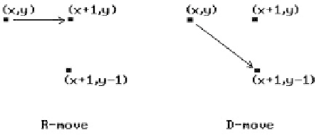
and ends at (r/÷2,r/÷2). Note that in this octant as we move from one point to the next
the x-coordinate will always increase by 1 and the y-coordinate will either stay the
same or decrease by 1. Any other choice would not minimize E. The two cases are
illustrated in Figure 2.19. We shall call the two possible moves an
R-move
or a
D-move
, respectively.
As we move from point to point, we choose that new point which minimizes E.
However, we can save computation time by computing the new E incrementally. To
see this, suppose that we are at (x,y). Then the current E, E
cur
, is given by
Figure 2.19.
Moves in circle-generating
algorithm.