Graphics Reference
In-Depth Information
Approach 1:
We can use the tangent to
C
at
p
0
to guess another nearby point.
Approach 2:
We can use a triangulation of the domain, replace the function f by an
approximation g obtained via linear interpolation of the values of f at
the vertices of the triangulation, and then find the intersection of
C
with the edges of the triangulation.
Approach 1 is basically what we used in Section 2.5.2 and 2.9.2 to draw lines and
circles. If
v
is a tangent vector to
C
at
p
0
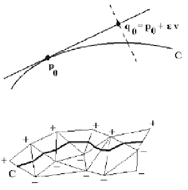
, we start with
q
0
=
p
0
+e
v
as a guess for the
next point on
C
and then adjust this guess to compensate for any deviation of
the contour from the tangent line. For example, we can look along the normal to the
tangent line at
q
0
to move back towards
C
. See Figure 14.27.
Of interest to us in this section is Approach 2 and the algorithm that is described
by Dobkin et al. in [DLTW90]. That paper also compares the two approaches. Roughly
speaking, Approach 1 produces an approximate solution using exact values of the
function and Approach 2 produces an exact solution using an approximation to the
function.
Because the complete algorithm described in [DLTW90], including handling of
various degenerate cases, is very lengthy, we only present an overview of it here and
refer the reader to the paper for the missing details. There is no loss of generality by
assuming that c = 0, and so our problem will be the following:
Given one point
p
0
with f(
p
0
) = 0, find the rest of the component
C
of the contour f
-1
(0) to
which
p
0
belongs.
The general idea of the algorithm is to triangulate the domain of f and to find the
points where the component intersects the edges of the triangles. The component is
then the polygonal curve obtained by connecting these intersection points with seg-
ments. See Figure 14.28. In essence we are solving the contour problem for an approx-
imation g to f, where g agrees with f on the vertices of the triangulation but is a linear
interpolation of the vertex values over the rest of each triangle. The advantages of this
approach are
Figure 14.27.
Tangent line approximation to a
contour.
Figure 14.28.
Connecting edge intersections.