Graphics Reference
In-Depth Information
ba
-
ab
10
10
c
=
1
2
a
0
...
Because u(t) = x(t), the parameterizations of the curve and its transform should be
taken either both in the positive or both in the negative t direction. From equation
(14.15) we see that —f(x
0
,y
0
) and —g(T
1
(x
0
,y
0
)) differ in the second coordinate by the
factor x
0
. We therefore use the sign of x
0
to decide whether the tracing direction with
respect to —g needs to be changed. Putting all this together, we determine the orien-
tations for tracing as follows:
(1) Assume the current tracing direction at (x,y) with respect to f is d(-f
y
,f
x
), where
d =±1.
(2) If we switch to tracing g, then trace g in direction xd(-g
y
,g
x
), that is, we use
g's standard trace direction if and only if xd > 0.
(3) When we finally are ready to switch back to tracing f, if we are tracing in direc-
tion d(-g
y
,g
x
), then start tracing in direction xd(-f
y
,f
x
).
To apply the above steps to f (x,y) = y
2
- x
2
- x
3
and show how
14.5.1.3
Example.
the problem indicated in Figure 14.25 disappears.
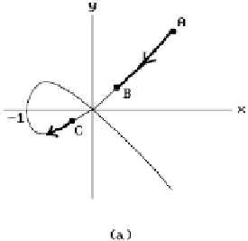
Solution.
See Figure 14.26 ([Hoff89]). If we start our tracing at
A
moving toward
the singularity at the origin, we eventually get to
B
where we switch to the transform
g and the curve v
2
- 1 - u = 0. We start at the point
B
1
on that curve and then trace
in direction (-g
y
,g
x
) until we get to point
C
1
at which time we have passed the singu-
larity and revert to tracing f at
C
, but with tracing direction (f
y
,-f
x
).
One common problem for all methods that try to compute an implicitly defined
set of points is to make sure that we end up with a set that has the correct topology.
Note that we ran into a similar problem in the last chapter in the context of finding
the intersection of two surfaces. Great strides have been made in the efficient appli-
cation of algebraic geometry to this issue. One example of this is the paper [GonN02],
where one can also find references to additional work.
Figure 14.26.
Adjusting the tracing direction at a singularity.