Graphics Reference
In-Depth Information
metric properties and relatively low degree (when compared with the popular cubic
splines) make them attractive for use in designing shapes such as fonts. Because of
this, a great deal of effort has been spent on devising efficient algorithms for com-
puting them. We shall look at a few of these in Sections 2.9.2 and 2.9.3.
Because one common theme of some of the algorithms that generate discrete
curves is derived from the geometric approach to solving differential equations, we
start with that subject.
2.5.1
Digital Differential Analyzers
Consider the basic first order differential equation of the form
(
)
dy
dx
gxy
hxy
,
,
=
(
)
=
fxy
,
.
(2.1)
(
)
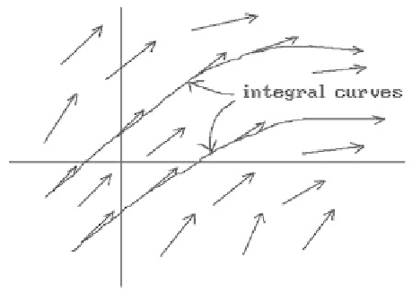
If y(x) is any solution, then f(x,y(x)) specifies the slope of the graph of y(x) at the point
(x,y(x)). In other words, if one thinks of the function f as specifying a
vector field
over
the entire plane (to (x,y) in the plane we associate the vector (1,f(x,y))), then solving
equation (2.1) corresponds to finding a parameterized curve x Æ (x,y(x)) whose
tangent vectors agree with the vectors from this vector field. Mathematicians call such
curves “integral curves.” In general, given a vector field, a curve whose tangent vectors
agree with the vectors of that vector field at every point on the curve is called an
inte-
gral curve
for that vector field. See Figure 2.7. The reason for this nomenclature is
that solving for the curve basically involves an integration process.
This idea of vector fields and integral curves leads to the following approach to
finding numerical solutions to differential equations called
Euler's method
. Suppose
that we want the solution to pass through
p
0
= (x
0
,y
0
). Since we know the tangent
vector to the solution curve there and since the tangent line is a good approximation
to the curve, moving a small distance along the tangent, say by e(h(x
0
,y
0
),g(x
0
,y
0
)),
where e is a small positive constant, will put us at a point
p
1
= (x
1
,y
1
), which hope-
fully is not too far away from an actual point on the curve. Next, starting at
p
1
we
repeat this process. In general, let
Figure 2.7.
Integral curves of a vector
field.