Graphics Reference
In-Depth Information
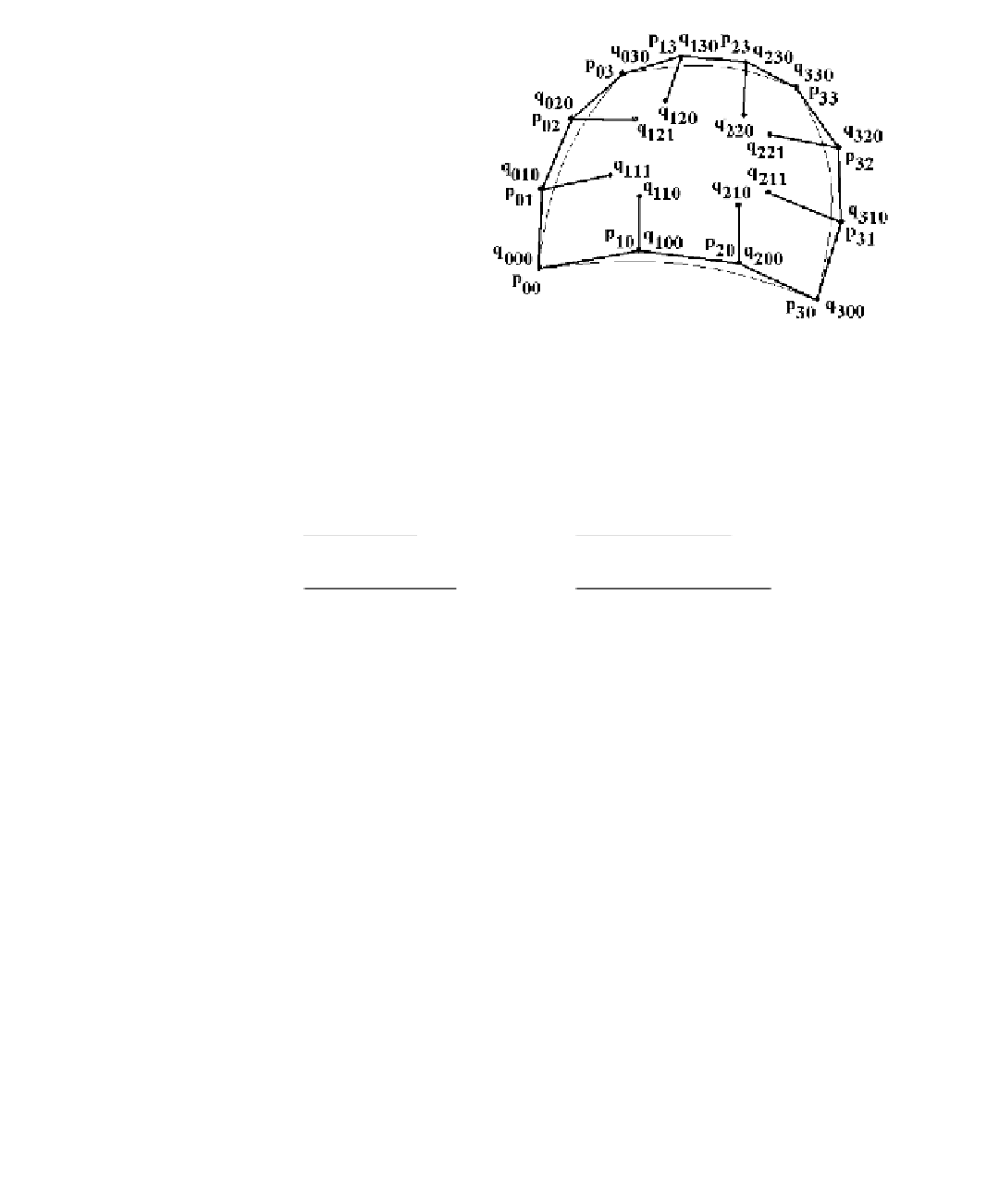
Figure 12.18.
The Gregory patch.
cubic Bézier patch, a Gregory patch uses 20 by splitting the interior four points
in two.
Let
q
ijk
Œ
R
3
, 0 £ i, j £ 3, k Œ {0,1}, and assume that
q
ij0
=
q
ij1
, (i,j) π (1,1), (2,1),
(1,2), (2,2). Define points
p
ij
(u,v) by
(
)
==
()
π
()()()( )
p
uv
,
q
q
ij
,
11
,, ,, , , , ,
21
1 2
2 2
1
ij
ij
0
ij
1
,
(
)
u
q
v
uv
+
+
q
-
u
q
+
-+
v
uv
q
110
111
210
211
(
)
=
(
)
=
p
uv
,
,
p
uv
,
,
11
21
1
(
)
(
)
(
)
u
q
v
uv
+-
1
1
q
1
-
u
q
v
uv
+-
1
q
120
121
220
221
(
)
=
(
)
=
p
uv
,
,
p
uv
,
.
12
22
+-
1
-+-
1
See Figure 12.18. Note the similarity between the the last four points and those used
in matrix (12.30) for the Gregory square.
Definition.
The parametric surface p(u,v) defined by
3
3
Â
Â
(
)
=
()
() (
)
puv
,
B
uB
v
p
uv
,
(12.44)
i
,
3
j
,
3
ij
i
=
0
j
=
0
for 0 £ u,v £ 1 is called a
Gregory patch
and the points
q
ijk
are called its
control points
.
The Gregory patch has a number of useful properties:
(1) If
q
ij0
=
q
ij1
, i,j Œ {1,2}, then it reduces to the ordinary cubic Bézier surface as
defined by equation (12.43).
(2) Using equation (12.44) makes evaluating p(u,v) and its derivatives just as easy
as the corresponding task for Bézier surfaces. The only extra work is that one
has to evaluate the interior points
p
ij
(u,v), i,j Π{1,2}, first.
(3) The surface lies in the convex hull of its twenty control points.
(4) It can be used to interpolate not only arbitrary Bézier boundary curves but
arbitrary “normal” derivatives along the boundary by choosing the interior
control points appropriately because