Graphics Reference
In-Depth Information
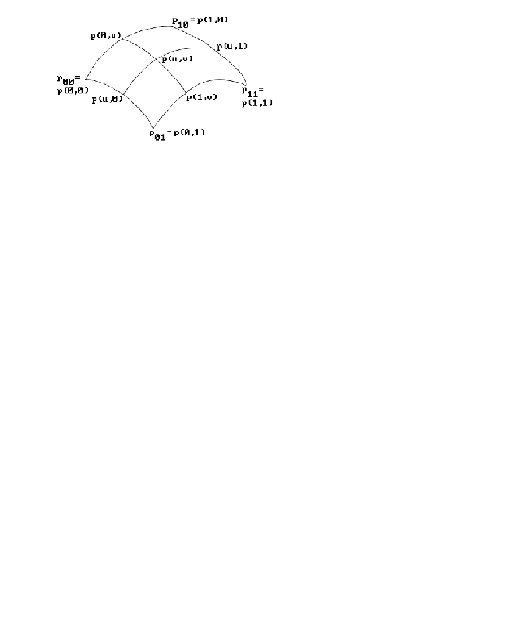
Figure 12.11.
A Coons patch.
as car bodies or airplane fuselages, that do not. In these situations, a common
approach is to divide the surface into patches defined by a network of curves. Each
patch is then parameterized by “filling in” or interpolating the given parameteriza-
tions of their boundary. The boundary curves themselves would have been defined by
an interpolation of data that comes from measurements on a model. In this section
we describe some general methods for defining surfaces that match some given
boundary data. Such parameterizations are sometimes called
transfinite interpolants
in the literature because one is interpolating an
infinite
set of points. All of the inter-
polation problems that we discussed previously (except for the case of lofted surfaces)
only interpolated a
finite
set of points. Finally, the boundary data may involve more
than just the curves however if one wants adjacent patches to meet in a smooth way.
To state our goal more precisely: it is to find a parameterization p(u,v), u,v Π[0,1],
that interpolates the four given boundary curves p(0,v), p(1,v), p(u,0), and p(u,1). See
Figure 12.11. A well-known solution to this problem is due to Coons ([Coon67]). His
approach builds on the lofted surface parameterizations for the boundary curve pairs
p(u,0), p(u,1) and p(0,v), p(1,v). Define operators P
1
and P
2
on a function of two vari-
ables p(u,v) by
(
)(
)
=-
(
) (
)
+
()
Pp u v
,
1
u p
0
,
v
up
1
,
v
,
(12.19a)
1
(
)(
)
=-
(
) (
)
+
()
Pp uv
,
1
vpu
,
0
vpu
,
1
.
(12.19b)
2
Compare the formulas for P
1
p and P
2
p with equation (12.13). These functions inter-
polate the boundary curves in the v- and u-direction, respectively. If our boundary
curves are straight lines parameterized in the standard linear way, then we would find
that we simply have the bilinear surface defined by equations (12.17) and P
1
p(u,v) and
P
2
p(u,v) are the same functions. If the boundary curves are not straight lines however,
then P
1
p(u,v) and P
2
p(u,v) are not the same, nor do they interpolate the other bound-
ary curves in the u- and v-direction, respectively. See Figure 12.12. For example, the
differences between P
1
p and the actual values of p along the u-direction boundaries
are
(
)
-
(
)
p u
,
0
P p u
,
0
and
1
(
-
()
pu
,
1
Ppu
,
1
.
1