Graphics Reference
In-Depth Information
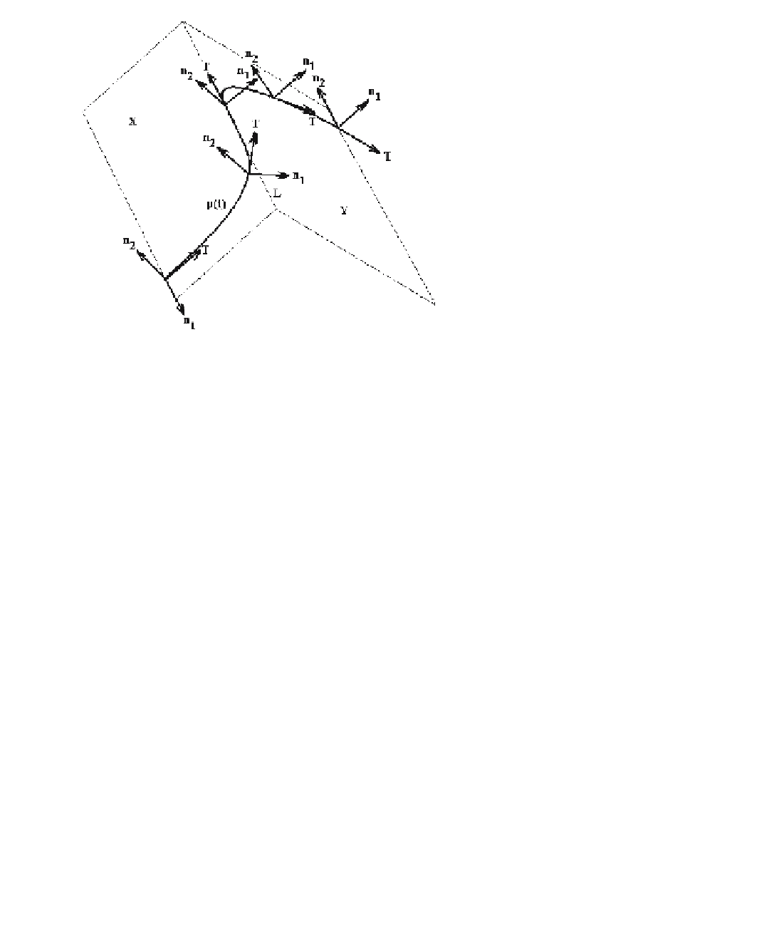
Figure 11.40.
Parallel transport
frames (T,n
1
,n
2
).
q
i
be the angle between T(t
i-1
) and T(t
i
) and let
w
i
= T(t
i-1
) ¥ T(t
i
) be the unit vector
that is orthogonal to the plane generated by T(t
i-1
) and T(t
i
). Then F(t
i
) =
(T(t
i
),n
1
(t
i
),n
2
(t
i
)) is the frame obtained by rotating (T(t
i-1
),n
1
(t
i-1
),n
2
(t
i-1
)) about
w
i
through an angle q
i
. See Figure 11.40.
To describe the mathematics behind this algorithm we need to use some facts
about frame fields on
R
3
and along curves. For the rest of this section we shall assume
that
[
]
Æ
R
3
pab
:,
is a regular space curve.
Definition.
A
vector field along the curve
p(t) is a vector-valued function
X
: [a,b] Æ
R
3
. The vector field X is
tangential
or
normal to p(t)
if the vectors
X
(t) and p¢(t) are
parallel or orthogonal, respectively, for all t.
Definition.
A normal vector field
X
along the curve p(t) is said to be
relatively par-
allel
to p(t) if
X
¢(t) is a tangential vector field.
In the case of a relatively parallel normal vector field
X
the fact that
X
•
X
¢=0
implies that the vectors
X
(t) have constant length. Although the next fact is not needed
here, it is an interesting connection to parallel curves that is worth making.
11.13.1 Theorem.
A normal vector field
X
is relatively parallel to p(t) if and only
if p(t) and q(t) = p(t) + X(t) are parallel curves.
Proof.
See [Bish75].
The next lemma answers the question as to whether relatively parallel normal
vector fields exist.