Graphics Reference
In-Depth Information
which can be written in the form
p
p
p
p
Ê
ˆ
0
Á
Á
Á
˜
˜
˜
()
=
(
)
1
32
qu
uuu
1
LM
,
(11.127)
c
2
Ë
¯
3
where
3
2
Ê
ˆ
(
)
(
)
2
(
)
3
1
-
c
3 1
c
-
c
3
c
1
-
c
c
Á
Á
Á
˜
˜
˜
2
(
)
(
)
2
0
1
-
c
2 1
c
-
c
c
L
c
=
.
0
0
1
-
c
c
Ë
¯
0
0
0
1
Define points
q
i
by the equation
q
q
q
q
p
p
p
p
Ê
ˆ
Ê
ˆ
0
0
Á
Á
Á
˜
˜
˜
Á
Á
Á
˜
˜
˜
1
1
-
1
=
MLM
,
c
2
2
Ë
¯
Ë
¯
3
3
Then equation (11.126) will be satisfied in this case also and we are done.
What we have just accomplished is to represent the initial cubic curve p(u) in
terms of two curves, so that we now have twice as much control data to use in manip-
ulating the curve.
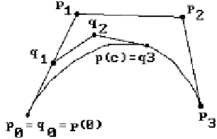
The cubic curve solution applies to cubic Bézier curves. In that case the matrix
M
is just the Bézier matrix. Figure 11.33 shows how p|[0,c] is now represented as a
Bézier curve with control points
q
0
,
q
1
,
q
2
, and
q
3
. Another four control points
q
3
,
q
4
,
q
5
, and
q
6
would represent p|[c,1]. This means that we can now use seven control
points to modify the curve, where before we had only four.
A more interesting problem is the general Bézier curve p(u) with control points
p
0
,
p
1
,...,
p
n
. It might seem as if the obvious solution here is simply to let a user
pick more control points interactively. The problem with that is that the user is then
Figure 11.33.
Subdividing cubic Bézier curves.