Graphics Reference
In-Depth Information
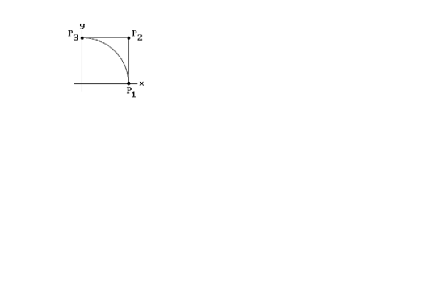
Figure 11.29.
The circle as a rational B-spline.
The Bézier approach to describing this curve is to look for three homogeneous control
points
P
1
,
P
2
, and
P
3
so that
(
)
()
=-
2
(
)
2
Pu
1
u
P
+-
2
u
1
u
P
+
u
P
1
2
3
(
)
+
2
(
)
(11.106)
=+
P
2
u
P
-
P
u
P
-
2
P
+
P
.
1
2
1
3
2
1
Equating the coefficients of the u's in the two equations (11.105) and (11.106) for P(u)
gives that
=
(
)
=
(
)
=
(
)
P
10 01
,,, ,
P
1101
,,, ,
and
P
0 20 2
,,, .
1
2
3
The corresponding
p
i
are shown in Figure 11.29(a). Using these
P
i
as control points
and the knot vector (0,0,0,1,1,1) gives us the NURBS curve that describes the first
quadrant of the unit circle. A NURBS representation for the second quadrant can
easily be obtained from this one by rotating the control points about the y-axis by
180 degrees. Alternatively, reparameterizing to [1,2], a parameterization q(u) for this
second quadrant is
2
-
( )
-+
Ê
Á
uu
uu
-+
-+
43
45
u
uu
22
45
ˆ
˜
Œ
[]
()
=
qu
,
,
for
u
12
,
,
2
2
and we can solve for the new control points as before. At any rate, the new control
points are
=
(
)
(
)
(
)
P
0202
,,, ,
P
=-
1101
,,, ,
and
P
=-
1001
,,,
3
4
5
Finally, rotating our control points by 180 degrees about the x-axis gives us the com-
plete NURBS representation for the whole unit circle. It is easy to check that the
parameterization can be written in the form
9
Â
()
wN
u
p
ii
,
3
i
()
=
i
=
1
pu
,
9
Â
()
wN
u
ii
,
3
i
=
1