Graphics Reference
In-Depth Information
Figure 11.24.
The de Boor algorithm for
B-splines using blossoms.
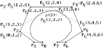
Figure 11.25.
Computing Bézier points
from the de Boor points.
Figure 11.24 shows how Algorithm 11.5.2.2 computes the value of the cubic B-spline
p(u) with knot vector (0,0,0,0,1,2,4,5,6,6,6,6) at u = 3. In that case, i = 5 and p(3) =
P
5
(3,3,3).
There is more geometry hidden in the formalism above. Given a blossom we can
use equations (11.90) and (11.96) to define the Bézier and de Boor points, respectively.
In other words, we have a way to switch between a Bézier and a B-spline represen-
tation for a B-spline curve. We show how this works with an example.
11.5.2.11 Example.
Let p(u) be a cubic B-spline p(u) with knot vector (t
i
) =
(0,0,0,0,1,2,4,5,6,6,6,6) and consider the interval [2,4]. Using the notation of Theorem
11.5.2.9 that interval corresponds to the values j = 5, k = 4, and 2 £
£ 5. In equation
(11.90) we would have d = 3. Using the blossom of the curve p(u) over [2,4] = I
5
=
[t
5
,t
6
] we can compute both the associated de Boor points
p
2
= P
5
(0,1,2),
p
3
= P
5
(1,2,4),
p
4
= P
5
(2,4,5), and
p
5
= P
5
(4,5,6) and the Bézier points
b
0
= P
5
(2,2,2),
b
1
= P
5
(2,2,4),
b
2
= P
5
(2,4,4), and
b
3
= P
5
(4,4,4). See Figure 11.25. From this it is easy to see the rela-
tionship between the Bézier and de Boor points. Consider the three points
p
3
=
P
5
(1,2,4) = P
5
(t
4
,t
5
,t
6
),
b
1
= P
5
(2,2,4) = P
5
(t
5
,t
5
,t
6
), and
p
4
= P
5
(5,2,4) = P
5
(t
7
,t
5
,t
6
). Using
barycentric coordinates and the linearity of P
5
with respect to its first coordinate, we
see that
t
-
-
t
t
-
-
t
75
74
54
74
=
(
)
+
()
b
=
p
+
p
34
p
14
p
.
1
3
4
3
4
t
t
t
t
Similarly,
b
2
= P
5
(4,2,4) = P
5
(t
6
,t
5
,t
6
), and