Graphics Reference
In-Depth Information
p
3
p
4
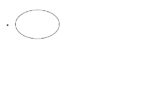
Figure 11.19.
A closed cubic uniform B-spline curve for
n
=
5.
p
2
p
5
p
0
p
1
and
¢
()
=-
+
q
i
1
1
pp
,
i
i
we also see that the first and last segment of the control polygon are tangent to the
curve at the first and last point, respectively.
There is a trick one can use to force a uniform B-spline to start at the first control
point and end at the last one to mimic the clamped uniform case. Qne can add some
“phantom” endpoints. One defines
p
=
2
p
-
p
and
p
=
2
p
-
p
.
(11.84)
-
1
0
1
n
+
1
n
n
-
1
See [BaBB87].
Next, we look at closed B-spline curves. The uniform B-spline curves come in
handy here. However, to close a curve we have to do more than simply add the first
point to the end of the control point sequence. Figure 11.19 shows a closed cubic
uniform B-spline curve with control points (
p
0
,
p
1
,
p
2
,
p
3
,
p
4
,
p
5
,
p
0
,
p
1
,
p
2
). A simple mod-
ification to formulas (11.78) and (11.81) leads to the following formulas for closed
curves. Let 1 £ i £ n + 1 and u Œ [0,1].
The closed quadratic uniform B-spline curve:
p
p
p
Ê
ˆ
(
)
i
-
1
mod
n
+
1
()
=
(
)
2
Á
Á
˜
˜
.
(11.85)
qu
uu
1
M
(
)
i
s
2
i
mod
n
+
1
Ë
¯
(
)
i
+
1
mod
n
+
1
The closed cubic uniform B-spline curve:
p
p
p
p
Ê
ˆ
(
)
i
-
1
mod
n
+
1
Á
Á
Á
˜
˜
˜
(
)
()
=
(
)
i
mod
n
+
1
32
qu
uuu
1
M
.
(11.86)
i
s
3
(
)
i
+
1
mod
n
+
1
Ë
¯
(
)
i
+
2
mod
n
+
1
Before we leave the subject of B-splines as matrices, we should point out that,
although this is an efficient way to compute them, the disadvantage to using these
matrices in a program is that it would involve code for lots of special cases. For
that reason and the fact that computers are powerful enough these days, a general