Graphics Reference
In-Depth Information
N
4,3
N
0,3
1
1
N
0,3
N
1,3
N
2,3
N
2,3
N
1,3
N
3,3
knots = (0,1,2,3,4,5)
knots = (0,0,0,1,2,3,3,3)
(a)
(b)
N
4,3
N
4,3
N
2,3
N
0,3
N
0,3
1
1
N
2,3
N
3,3
N
1,3
N
3,3
N
1,3
knots = (0,0,0,1,9,2,3,3)
knots = (0,0,0,1,1,3,3,3)
(c)
(d)
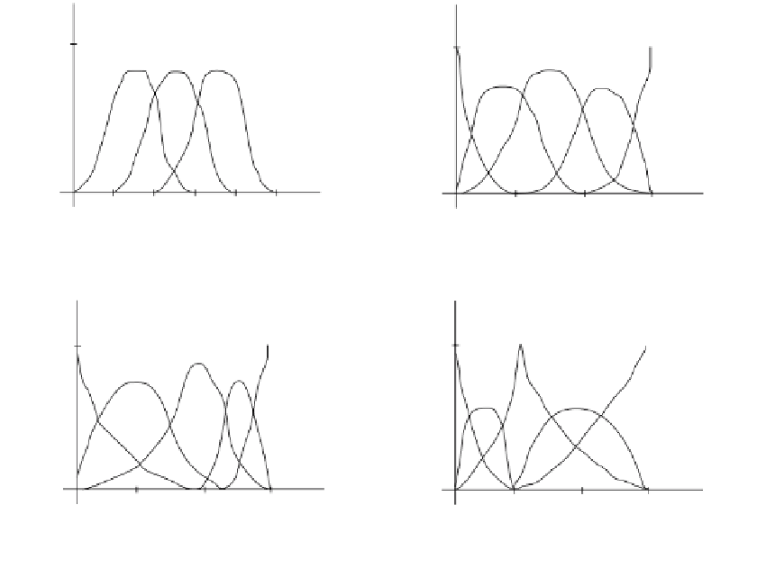
Figure 11.16.
Some quadratic B-splines.
Because of the importance of B-spline curves to geometric modeling, much effort
has gone into coming up with efficient algorithms for computing them and their deriv-
atives. We leave the discussion of these algorithms to Section 11.5.4, at which time
we will also be able to include the rational B-spline curves. In this section will shall
only consider some special ways of computing and working with the quadratic and
cubic curves which, hopefully, will aid the reader in understanding the general curves.
Consider Figure 11.16, which shows some quadratic B-splines. Note how nice and
symmetric the curves look in Figure 11.16(a) and (b) when the knots are spaced evenly
and how this symmetry is lost in Figure 11.16(c) and (d) when the knot spacing
becomes irregular. The cusp in Figure 11.16(d) is caused by the knot 1 which has
multiplicity 2. Figure 11.17 shows all the clamped uniform cubic B-splines N
i,4
(u)
associated to the knot vector (0,0,0,0,1,2,3,4,5,6,6,6,6). Again we have regularly
spaced knots and symmetric curves.
The fact is that over uniformly spaced knots the B-splines of a given degree all
have the same shape and are just translates of each other. This is easy to see from the
definition of the N
i,k
(u). Assume we have a knot vector (0,1,2, . . .), so that u
i
= i. A
simple induction shows that