Curves in Computer Graphics - Computer Graphics and Geometric Modeling - page 401

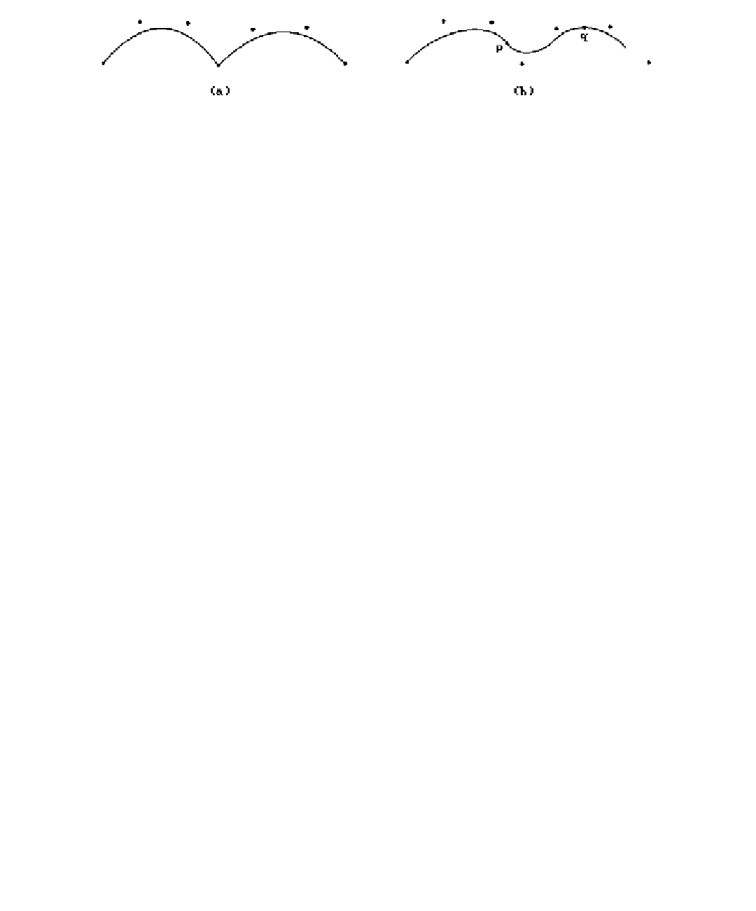
Figure 11.11. Bezier curves.

(1) The degree of the curve increases with the number of control points.
(2) There is no local control. The smallest change in any control points forces a
recomputation of the whole curve, although the further that one is from the
control point that was changed, the smaller is the change in the curve.

The usual way to avoid the first disadvantage is to use piecewise Bézier curves, but
then one has to worry about the overall smoothness of the curve and whether the indi-
vidual pieces fit together nicely. There are tricks that one can play to preserve visual
smoothness, however. For example, by taking four control points at a time, one can
get a piecewise cubic Bézier curve. If the last edge of one four-point control polygon
is parallel to the first edge of the next control polygon, then the curve will look smooth
without any apparent corner. To achieve this one can add control points to the orig-
inal set that are the midpoints of appropriate segments. Figure 11.11(a) shows two
four-point Bézier curves that meet in a corner. By adding the points p and q , the new
curve in Figure 11.11(b), which now consists of three four-point Bézier curves, no
longer has a corner. Of course, adding points means that one has changed the curve
that a user is trying to design, but the change will probably not be noticeable. Besides,
in an interactive environment, a user may not have a specific curve in mind anyway
and is only interested in being able to control the general shape.

11.5. B-Spline Curves

11.5.1. The Standard B-Spline Curve Formulas

One common problem with the curves discussed so far is that any change to a control
point forces recomputation of the whole curve. This is very undesirable. B-spline
curves solve this problem. Changes to control points will have only a local effect on
the curve.
B-splines can be defined in several ways. One can define them using

(1) a “brute force” approach by solving equations specifying certain constraints
(see Theorem 11.5.1.1 for example),
(2) truncated (also called one-sided ) power functions (see [deBo78] or [BaBB87]),
(3) recursion (the functions N i,k (u) defined later in this section),
(4) matrices (typically for the case of quadratic and cubic B-splines), or
(5) a multiaffine map approach (see Section 11.5.2).