Graphics Reference
In-Depth Information
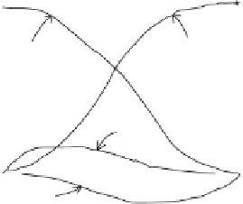
Figure 11.5.
The Hermite basis functions.
1
F
2
F
1
F
3
1
F
4
More importantly,
()
=
()
+
()
+
()
+
()
px
y F x
yF x
m F x
mF x
.
(11.15)
01
12
03
14
Notice that the polynomials F
i
(x) satisfy
()
=
()
=
¢
()
=
¢
()
=
F
01
,
F
10
,
F
00
,
F
10
,
1
1
1
1
()
=
()
=
¢
()
=
¢
()
=
F
00
,
F
11
,
F
00
,
F
10
,
2
2
2
2
()
=
()
=
¢
()
=
¢
()
=
F
00
,
F
10
,
F
01
,
F
10
,
3
3
3
3
()
=
()
=
¢
()
=
¢
()
=
F
00
,
F
10
,
F
00
,
F
11
.
(11.16)
4
4
4
4
Figure 11.5 shows the graph of these functions. The existence of functions with these
properties would by itself guarantee that equation (11.15) is satisfied.
Definition.
The matrix
M
h
defined by equation (11.10) is called the
Hermite matrix
.
The polynomials F
i
(x) defined by equations (11.13) and (11.14) are called the
Hermite
basis functions
.
For future reference, note that the equation
()
+
()
=
Fx F x
1
(11.17)
1
2
holds for all x. Also, because the F
i
are part of a more general pattern of functions
similar to that of the Lagrange polynomials, we introduce the following alternate nota-
tion for them:
HFHFHF dHF
=
,
=
,
=
,
=
.
(11.18)
03
,
1
13
,
3
23
,
4
33
,
2
This notation will be useful in the next chapter.
Lemma 11.2.2.1 is a special case of a general interpolation problem.
The piecewise Hermite interpolation problem:
Given triples (x
0
,y
0
,m
0
), (x
1
,y
1
,m
1
),...,
and (x
n
,y
n
,m
n
), find cubic polynomials p
i
(x), i = 0,1,..., n - 1, so that