Graphics Reference
In-Depth Information
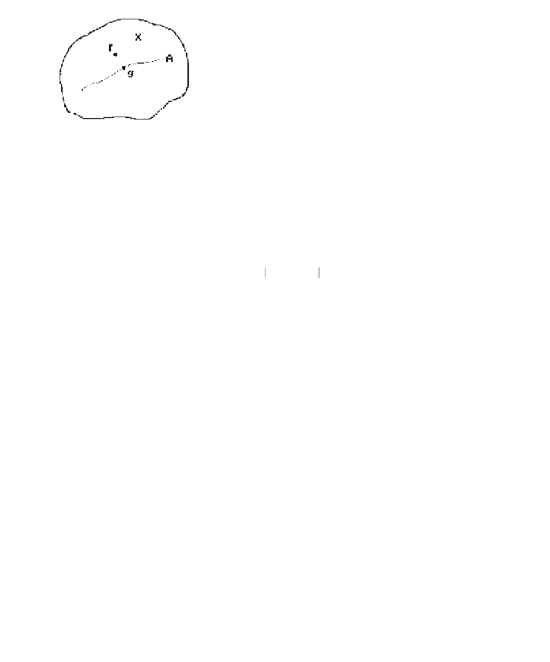
Figure 11.2.
The general approximation problem.
(1) The function g should be “close” to f with respect to some appropriate metric.
(2) The coefficients c
i
should be unique.
What does it mean for functions to be close? Well, that depends on the metric that
is chosen for the function spaces in question (see Section 5.2 in [AgoM04]). Many
metrics are possible and one needs to choose the one that is appropriate for the
problem at hand. A common metric is the so-called “max” metric where d(a,b), the
distance between two functions a(
x
) and b(
x
), is defined by
Ú
(
)
=
()
-
()
dab
,
a
x
b
x
d
x
.
D
On the other hand, the function f(
x
) may only be known at a finite number of points
x
1
,
x
2
,...,
x
s
, so that the best we can do is to minimize the error at the points
x
j
.
Before we define the well-known approach to the approximation problem in this
important special case, we make two observations. First, the function g defined
by equation (11.1) depends on the values c
i
and so we shall use the notation g(
x
;c
1
,
c
2
,...,c
k
) to indicate this dependence explicitly. Second, since distances involve a
square root, one simplifies things without changing the minimization problem by
using the square of the distance.
Definition.
The function g(
x
;c
1
,c
2
,...,c
k
) that minimizes
s
2
Â
(
)
=
(
()
-
(
)
)
Ec c
,
,...,
c
f
x
g
x
;
c c
,
,...,
c
12
k
j
j
12
k
j
=
1
is called the
least squares approximation
to the function f(
x
).
Finding the least squares approximation involves setting the partials ∂E/∂c
i
to zero
and solving the resulting system of linear equations for the c
i
.
When dealing with approximation problems one usually encounters other con-
straints. Some of these are:
(1) Interpolatory constraints:
()
=
(
,
g
x
f
x
for some fixed points
x
.
j
j
j