Graphics Reference
In-Depth Information
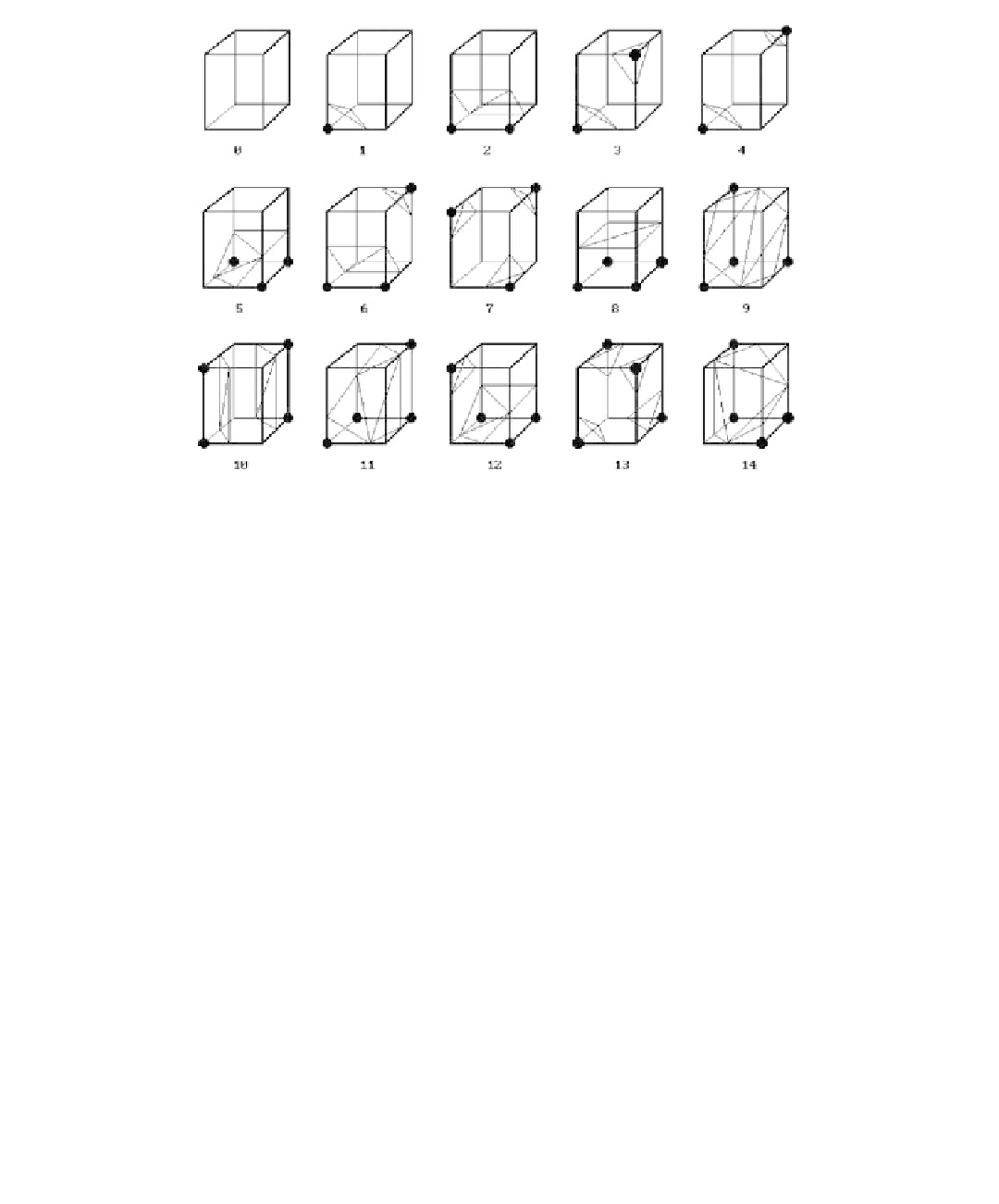
Figure 10.19.
The marching cube algorithm cases.
[LorC87] applied the marching cube algorithm to three-dimensional medical data
that provided two-dimensional slices of data. They used the following steps to create
a surface from this data:
(1) Four slices of data were read into memory at a time.
(2) Two slices were scanned to create a cube from four neighbors on one slice and
four neighbors on the next slice.
(3) By comparing the eight density values at the cube vertices with the surface
constant an eight bit (one bit per vertex) index was calculated.
(4) This index was used to look up in a precalculated table the edges of the cube
that are intersected by the surface.
(5) The actual surface-edge intersections are then computed by linear interpola-
tion of the density values at the cube vertices. The intersection is divided into
triangles.
(6) Central differences are used to compute a unit normal at each cube vertex
which are then interpolated to each triangle vertex.
(7) Finally, the triangle vertices and normals are output.
[LorC87] points out that linear interpolation is adequate and that using higher-degree
interpolants does not provide any significant improvement. Although one could deter-
mine normals from the surface triangles themselves, it turns out that the gradient
method used above gives substantially better results. In order to avoid aliasing prob-
lems, the initial data must have been sampled enough to produce sufficiently small
triangles in the surface.