Graphics Reference
In-Depth Information
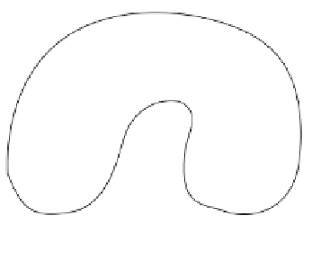
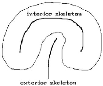
Figure 5.26.
Interior and exterior skeletons.
Most algorithms are basically discrete algorithms. One exception is the algorithm
described in [Hoff94] for CSG objects. In this regard, see also [LBDW92]. The authors
describe how one can obtain an approximation to a variant of the Voronoi diagram
for CSG objects. Sometimes bisectors of surfaces are rational. See [ElbK99]. In case
of polyhedra, the medial surface consists of bisectors that are planes or quadric sur-
faces. An algorithm for planar regions with curved boundaries can be found in
[RamG03].
To use the medial axis representation effectively one needs to know not only how
to compute it but also how one can reconstruct the original object from it. The latter
task is often referred to as
refleshing
. Algorithms for refleshing divide into direct and
implicit approaches.
The
direct approach
to refleshing tries to reconstruct the boundary surface of
the original object directly using the given radius or distance function. This amounts
to constructing the surface from a variable offset type surface. See [GelD95]. Self-
intersections are a problem with offsets and the exterior skeleton has been used here
to help prevent these. See [STGLS97]. The
exterior skeleton
or
exoskeleton
of an object
is the skeleton of the complement of the object. The ordinary skeleton is sometimes
called the
interior skeleton
or
endoskeleton
. The exterior skeleton comes in handy at
those places where the boundary of the object is concave. See Figure 5.26.
The
implicit approaches
to refleshing try to define the boundary surface implic-
itly as the zero set of a suitable function. They can be further subdivided into those
that use a distance function and those that use convolution methods. See [BBGS99]
for a more detailed discussion of this along with references. The paper also describes
a new distance function approach. This involves triangulating the medial axis and
defining a local distance function for each triangular facet. The global distance func-
tion is then the minimum of all the local ones. To give the reader a flavor of how a
local distance function is constructed, we sketch the construction in the case where
the radius function is constant over a facet. The local distance function is a compos-
ite of functions defined over regions that are related to the Voronoi cells associated
to the facet, its edges, and its vertices. See Figure 5.27, which shows a triangular facet
with vertices
p
1
,
p
2
, and
p
3
and its associated Voronoi cells whose boundaries are
obtained by sweeping a vector orthogonal to the edges of the facet orthogonally to the
plane of the facet. Let f
si
be the local distance function for point
p
i
determined by the