Graphics Reference
In-Depth Information
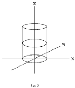
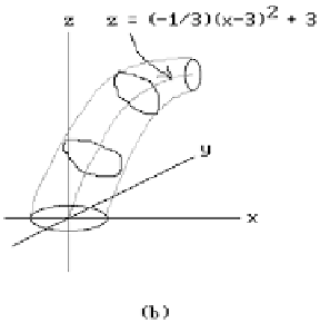
Figure 5.20.
Generative models.
See Figure 5.20(a). A more interesting example is shown in Figure 5.20(b) where we
use
v
1
3
Ê
Ë
ˆ
¯
Ê
Ë
ˆ
¯
2
(
)
=-
()
+
(
)
f
p
,
v
1
R
p
v
,
0
,
-
x
-
33
+
v
6
and R
v
is the rotation about the y-axis in
R
3
through an angle of pv/6. This corre-
sponds to sweeping the unit circle along the parabola
1
3
2
(
)
z
=-
x
-
33
+
in the xz-plane. The circle gets rotated and scaled by a factor of 1 - v/6 as we move
it.
The parameterization S(u,v) in equation (5.3) can be thought of as defining a one-
parameter family of curves g
v
defined by g
v
(u) = f (g(u),v). As the examples in Figure
5.20 suggest, this family of curves can correspond to a fixed curve being operated on
by quite general transformations as it is swept along arbitrary curves. This is, in fact,
one reason for creating the generative model representation, namely, that it allows
powerful operators for modifying objects.
More generally, generative models of arbitrary dimension have parameterization
S(u,v) of the form
k
s
k
+
s
n
S
:
RR
¥=
R
Æ
R
(
)
(
()
)
(5.4)
uv
,
Æ
TFu v
,
,
where F :
R
k
Æ
R
m
and T :
R
m
¥
R
s
Æ
R
n
. This is thought of as a (k + s)-dimensional
model obtained by sweeping a k-dimensional object along an s-dimensional path. For
example, this allows us to define solids as generative models. A common representa-
tion is to represent a solid as sweeping an area along a curve.