Parallel Computing for Bayesian Networks - Bayesian Networks in R: With Applications in Systems Biology - page 109

14

12

10

8

6

1 2 3 4 5 6

number of slaves

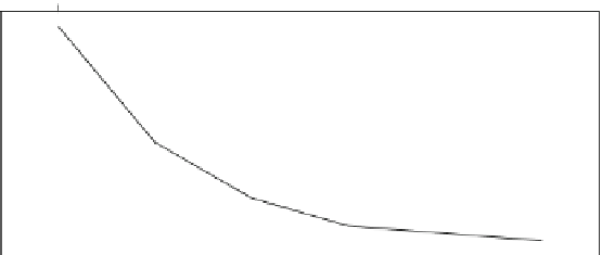
Fig. 5.2 Performance of the Grow-Shrink algorithm for different numbers of slave processes,
measured by its execution time (in seconds)

As we can see from the output of clusterEvalQ , the first slave process per-
formed 2,698 (41

. .

21 %). Only
4 tests were performed by the master process. The difference in the number of tests
between the two slaves is due to the topology of the network; different nodes have
Markov blankets and neighborhoods of different sizes, which require different num-
bers of tests to learn.
Increasing the number of slave processes reduces the number of tests performed
by each slave, further increasing the overall performance of the algorithm.
> cl = makeCluster(3, type = "MPI")
3 slaves are spawned successfully. 0 failed.
> res = gs(hailfinder, cluster = cl)
> unlist(clusterEvalQ(cl, .test.counter))
[1] 1667 2198 2598
> stopCluster(cl)
> cl = makeCluster(4, type = "MPI")
4 slaves are spawned successfully. 0 failed.
> res = gs(hailfinder, cluster = cl)
> unlist(clusterEvalQ(cl, .test.counter))
[1] 1116 1582 1860 1905
> stopCluster(cl)
The execution times of the Grow-Shrink algorithm for clusters of 2, 3, 4, 5, and
6 slaves are reported in Fig. 5.2 . It is clear from the figure that the gains in execu-
tion time follow the law of diminishing returns —i.e., adding more slave processes
produces smaller and smaller improvements, up to the point where the increased
overhead of the communications between the master and the slave processes starts
actually degrading performance.
Another important consideration is whether the data set we are learning the
network from actually contains enough observations and variables to make the
use of the parallel implementation of a learning algorithm worthwhile. In fact,
for hailfinder the sequential implementation of the Grow-Shrink algorithm is
faster than the parallel one.

71 %) conditional tests, and the second one 3,765 (58