Biology Reference
In-Depth Information
0.6
low
high
0.4
0.2
0.0
6
8
10
expression level
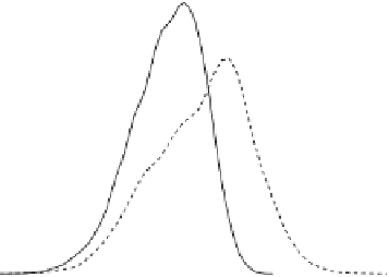
Fig. 4.3
Density plot of the expression levels of gene
265768 at
at time
t
for expression levels
of gene
245094 at
above 8 (
solid line
) and below 8 (
dashed line
) at time
t
−
1
> lasso.s = penalized(response = y, penalized = x,
+
lambda1 = lambda)
> coef(lasso.s)
(Intercept) 258736_at 257710_at 255070_at
-2.659077706 -0.009220815 0.273648262 -0.444106451
245319_at 245094_at1
-0.134050990 1.589716443
Here we are assuming that the dynamic Bayesian network is time-homogeneous,
since we are using the same data to fit both the variables at time
t
against the ones
at time
t
2.
Subsequently, we create the network structure for the dynamic Bayesian network
as we did in the previous example; the result is shown in Fig.
4.4
.
−
1 and the variables at time
t
−
1 against the ones at time
t
−
> dbn2 = empty.graph(c("265768_at", "245094_at",
+ "258736_at", "257710_at", "255070_at",
+ "245319_at", "245094_at1"))
> dbn2 = set.arc(dbn2, "245094_at", "265768_at")
> for (node in names(coef(lasso.s))[-c(1, 6)])
+ dbn2 = set.arc(dbn2, node, "245094_at")
> dbn2 = set.arc(dbn2, "245094_at1", "245094_at")
The easiest way to fit the parameters of
dbn2
is to estimate all of them via maximum
likelihood and then to substitute the parameters of
265768 at
and
245094 at
with the ones from the LASSO models
lasso.t
and
lasso.s
.
> dbn2.data = as.data.frame(x[, nodes(dbn2)[1:6]])
> dbn2.data[, "245094_at"] = y
> dbn2.data[, "245094_at1"] = x[, "245094_at"]
> dbn2.fit = bn.fit(dbn2, dbn2.data)


Search WWH ::

Custom Search