Information Technology Reference
In-Depth Information
(a)
µ
1
P(e)
N(e)
0
-L
L
(b)
(c)
µ
1
N
ZE
P
N(ce)
µ
1
P(ce)
-H
0
H
0
W
1
-L
L
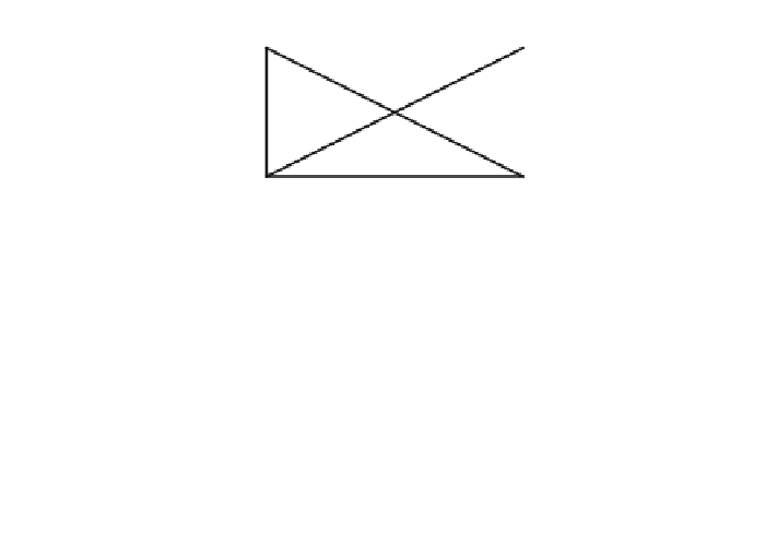
Fig. 9 Triangular membership functions of simplest FLC for a error, b change in error and
c output
δ
I
max
FLC, in a way that this cascaded combination (i.e., approximated FLC) maps the
output of a 49-rule FLC, with least square error. The output of approximated FLC
in terms of nth order polynomial of u
1
(k) is given as:
a
n
u
1
ð
a
n
1
u
n
1
1
u
2
ð
k
Þ
¼
k
Þþ
ð
k
Þþþ
a
1
u
1
ð
k
Þþ
a
0
ð
6
Þ
where, u
1
(k) and u
2
(k) are the outputs of 4-rule FLC and proposed approximated
FLC, respectively. a
0
,a
1,
a
2,
…
cients of nth order polynomial. The
block diagram of approximation scheme is shown in Fig.
10
.
Sum of square errors (SSE), at N data points is represented as:
a
n
are the coef
X
N
2
SSE
¼
1
f
u
ð
k
Þ
u
2
ð
k
Þg
ð
7
Þ
t
¼
X
N
t¼1
½
a
n
u
1
ð
a
n
1
u
n
1
2
ð
Þf
Þþ
ð
Þþþ
a
1
u
1
ð
Þþ
a
0
g
ð
8
Þ
SSE
¼
u
k
k
k
k
1
-
cients are equated to zero to get as many equations as the number of unknown
coef
To minimize SSE, its partial derivatives with respect to each unknown coeffi-
cients. The solution of these equations gives the values of these unknown
coef
cients. The
fl
ow chart, to
find the unknown coef
cients a
n
,a
n
−
1
,a
n
−
2
,
…
a
1
and
a
0
, of compensating polynomial, is shown in Fig.
11
.


Search WWH ::

Custom Search