Modeling, Identification and Control of Irrigation Station with Sprinkling: Takagi-Sugeno Approach - Complex System Modelling and Control Through Intelligent Soft Computations - page 472

If we factorize the Eq. 15 , we have:

yN

x T N

h ðÞ ¼h N ð N 1 Þþ GN ðÞ yN ðÞ ðÞ h ð N 1 Þ ðÞ ð 20 Þ

3.4 Application of FCM Algorithm on the Station
of Irrigation by Sprinkling

Let us consider a system described by the Eq. 6 . Firstly, we approximate the
nonlinear function Eq. 6 by the model of Takagi-Sugeno (TS):

R i and x kn is A in then y i a i x k þ

: if fix k1 isA i1 and x k2 is A i2 and ... ¼ b i ð 21 Þ

T

To represent the rule, we need use observations vector x k ¼ ½ x k1 ; x k2 ; ...; x kn

the units fuzzy A i1 ; A in to identify the parameters in the model 21 , we builds

the matrix of regression X and the vector of the output Y starting from measure-
ments

A i2 ; ...;

T and Y

resulting from the system such as: X ¼ x 1 ; x 2 ; ...; x N ¼

T with N

½ y 1 ; y 2 ; ...; y N n.

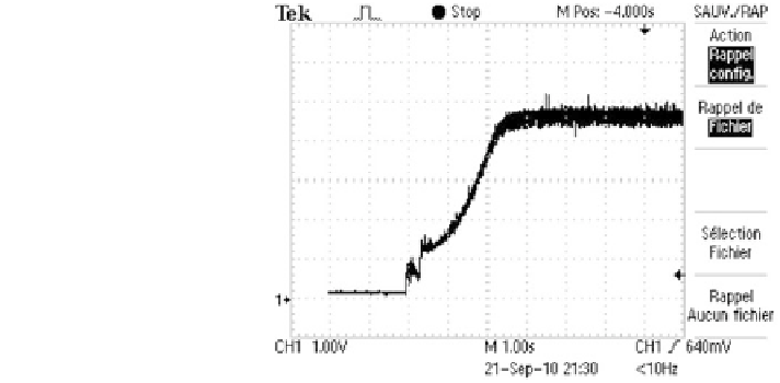
cation of T-S model parameters requires a taking away of the real
signals of irrigation station. Using a numerical oscilloscope, we took the real
dynamics of pressure and

The identi

fl flow of the station of irrigation by sprinkling, then

(Figs. 6 , 7 and 8 ):
These results are taken from connectors of the cabinet.
In order to initialize the iteration count l =0,we fix the weighting degree

m = 2.75 what makes it possible to initialize the partial random matrix U. We pass

Fig. 6 Real curve of the
pressure evolution