Information Technology Reference
In-Depth Information
consecutive observations than prune the ith hidden unit and
reduce the dimensionality of the related matrices
end
5. n = n + 1 and go to step 1.
if of
i
ðÞ
\
d
for
ʾ
6.2 Prediction Algorithm Results
Forecast algorithms performance have been evaluated through real experimental
tests based on data acquired from March 2012 to August 2012. In particular the 3
houses with 3.3 KWp PV plant considered, are located in Ripatransone (AP), Italy.
The MRANEKF learning algorithm starts with a pre-trained net based only on few
information found on the web, such as power production pro
le of clear sky days
and cloudy days for the speci
ed location Pvg (
2011
), panel orientation and tilting
and typical electrical load pro
le of a house. This is a common operating condition,
when no sensors and measures are available before the forecast begins.
The inputs of the production forecasting network, as shown in Fig.
10
, are:
the day of the year (from 1 to 365)
the hour of the day (considered from 0 to 24)
the ambient temperature (in Kelvin)
the sky clearness index (a coef
cient ranging from 0 to 10 mapping the website
“
”
“
”
forecast, e.g.
clear and sunny
is 10 while
clouds and heavy rain
is 0)
the wind speed (in m/s)
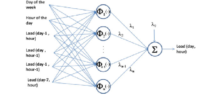
The input pattern of the consumption forecasting net, as shown in Fig.
11
,
consists of:
the day of the week (e.g. Monday is day 1, Tuesday is day 2)
the hour of the day (considered from 0 to 24)
Fig. 11 Input-output structure of the load forecast network

Search WWH ::

Custom Search