Geoscience Reference
In-Depth Information
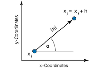
Fig. 7.17
Separation vector
h
between two points.
We then obtain the experimental variogram
G
, as half the squared dif erences
between the observed values:
G = 0.5*(Z1 - Z2).^2;
In order to speed up the processing we use the MATLAB capability to
vectorize commands instead of using
for
loops to run faster. However, we
have computed
n2
pairs of observations although only
n
(
n
-1)/2 pairs are
required. For large data sets (e.g., more than 3,000 data points) the sot ware
and physical memory of the computer may become limiting factors. In
such cases, a more ei cient method of programming is described in the
user manual for the SURFER sot ware (SURFER 2002). h e plot of the
experimental variogram is called the
variogram cloud
(Fig. 7.18), which we
obtain by extracting the lower triangular portions of the
D
and
G
arrays.
indx = 1:length(z);
[C,R] = meshgrid(indx);
I = R > C;
plot(D(I),G(I),'.' )
xlabel('lag distance')
ylabel('variogram')
h e variogram cloud provides a visual impression of the dispersion of values
at the dif erent lags. It can be useful for detecting outliers or anomalies, but it is
hard to judge from this presentation whether there is any spatial correlation,
and if so, what form it might have and how we could model it (Webster and
Oliver 2001). To obtain a clearer view and to prepare a variogram model the
experimental variogram is now replaced by the variogram estimator.
h e variogram estimator is derived from the experimental variograms in
order to summarize their central tendency (similar to the descriptive statistics
derived from univariate observations, Section 3.2). h e classical variogram