Geoscience Reference
In-Depth Information
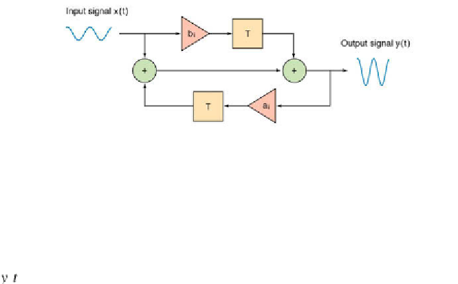
Fig. 6.2
Schematic of a linear time-invariant i lter with an input
x
(
t
) and an output
y
(
t
). h e
i lter is characterized by its weights
a
i
and
b
i
. and the delay elements
T
. Nonrecursive i lters
require only nonrecursive weights
b
i
whereas recursive i lters also require the recursive i lter
weights
a
i
.
with the known problems in the design of zero-phase i lters. h e larger of the
two quantities
M
, and
N
1
+
N
2
or
N
, is the order of the i lter.
We use the same synthetic input signal
x5
as in the previous example to
illustrate the performance of a recursive i lter.
clear
t = (1:100)';
rng(0)
x5 = randn(100,1);
h is input is then i ltered using a recursive i lter with a set of weights
a5
and
b5
,
b5 = [0.0048 0.0193 0.0289 0.0193 0.0048];
a5 = [1.0000 -2.3695 2.3140 -1.0547 0.1874];
m5 = length(b5);
y5 = filter(b5,a5,x5);
and the output
y5
corrected for the phase
y5 = y5(1+(m5-1)/2:end-(m5-1)/2,1);
y5(end+1:end+m5-1,1) = zeros(m5-1,1);
We can now plot the results.
plot(t,x5,'b-',t,y5,'r-')