Geoscience Reference
In-Depth Information
of the system. h e transitivity coei cient has its roots in graph theory and
characterizes the regularity or complexity of the system.
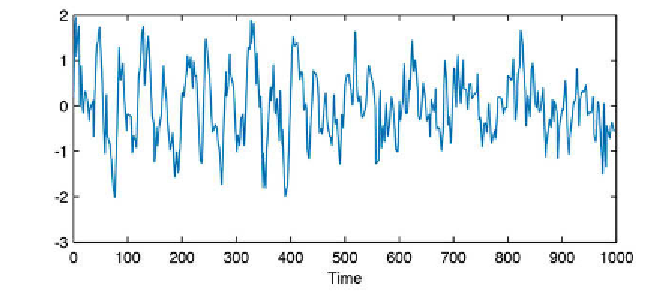
We load the synthetic time from the i le
series3.txt
, interpolate the data
to an annual time axis, and reconstruct its phase space trajectory using an
embedding dimension of 5 and a time delay of 3 (Fig. 5.26).
clear
series3 = load('series3.txt');
t = 0 : 1 : 996;
series3L = interp1(series3(:,1),series3(:,2),t,'linear');
plot(t,series3L)
xlabel('Time')
N = length(series3L);
tau = 3; m=5;
N2 = N - tau*(m - 1);
xe = zeros(N2,m);
for mi = 1:m
xe(:,mi) = series3L([1:N2] + tau*(mi-1));
end
Using the vectorized approach we calculate the recurrence plot by applying
a threshold of 1.2 to the distance matrix (Fig. 5.27).
x1 = repmat(xe,N2,1);
x2 = reshape(repmat(xe(:),1,N2)',N2*N2,m);
S = sqrt(sum((x1 - x2).^ 2,2));
S = reshape(S,N2,N2);
Fig. 5.26
Time series of the synthetic data used in the example of quantitative measures of
recurrence plots.