Geoscience Reference
In-Depth Information
We can now interpolate the two time series to this axis with
linear
and
spline
interpolation methods, using the function
interp1
.
series1L = interp1(series1(:,1),series1(:,2),t,'linear');
series1S = interp1(series1(:,1),series1(:,2),t,'spline');
series2L = interp1(series2(:,1),series2(:,2),t,'linear');
series2S = interp1(series2(:,1),series2(:,2),t,'spline');
In the
linear
interpolation method the linear interpolant is the straight line
between neighboring data points. In the
spline
interpolation the interpolant
is a piecewise polynomial (the
spline
) between these data points. h e
method
spline
with
interp1
uses a piecewise cubic spline interpolation, i.e.,
the interpolant is a third-degree polynomial. h e results are compared by
plotting the i rst series before and at er interpolation.
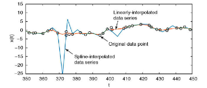
plot(series1(:,1),series1(:,2),'ko'), hold on
plot(t,series1L,'b-',t,series1S,'r-'), hold off
We can already observe some signii cant artifacts at ca. 370 kyrs. Whereas
the linearly-interpolated points are always within the range of the original
data, the spline interpolation method produces values that are unrealistically
high or low (Fig. 5.9). h e results can be compared by plotting the second
data series.
plot(series2(:,1),series2(:,2),'ko'), hold on
plot(t,series2L,'b-',t,series2S,'r-'), hold off
In this series, only a few artifacts can be observed. h e function
interp1
also
provides an alternative to
spline
, which is
pchip
. h e name
pchip
stands for
Fig. 5.9
Interpolation artifacts. Whereas the linearly interpolated points are always within
the range of the original data, the spline interpolation method results in unrealistic high and
low values.