Geoscience Reference
In-Depth Information
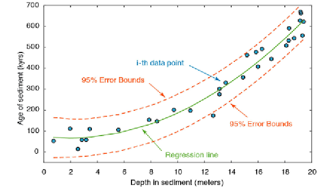
Fig. 4.8
Curvilinear regression from measurements of barium content. h e plot shows the
original data points (circles), the regression line for a polynomial of degree
n
=2 (solid line),
and the error bounds (dashed lines) of the regression.
plot(meters,polyval(p,meters),'r'), hold off
[p,s] = polyfit(meters,age,2);
[p_age,delta] = polyval(p,meters,s);
plot(meters,age,'o',meters,p_age,'g',meters,...
p_age+2*delta,'r--',meters,p_age-2*delta,'r--')
axis([0 20 -50 700]), grid on
xlabel('Depth in Sediment (meters)')
ylabel('Age of Sediment (kyrs)')
h e plot shows that the quadratic model for this data is a good one. h equality
of the result could again be tested by exploring the residuals, by employing
resampling schemes, or by cross validation. Combining regression analysis
with one of these methods provides a powerful tool in bivariate data analysis,
whereas Pearson's correlation coei cient should be used only as a preliminary
test for linear relationships.
4.10 Nonlinear and Weighted Regression
Many bivariate data in earth sciences follow a more complex trend than a
simple linear or curvilinear trend. Classic examples for nonlinear trends are
the exponential decay of radionuclides, or the exponential growth of algae
populations. In such cases, MATLAB provides various tools to i t nonlinear