Geoscience Reference
In-Depth Information
above),
rhos1000
has the dimensions of 1000-by-4, i.e., 1000 values for each
element of the 2-by-2 matrix. Plotting the histogram of the 1000 values for
the second element, i.e., the correlation coei cient of
(x,y)
, illustrates the
dispersion of this parameter with respect to the presence or absence of the
outlier. Since the distribution of
rhos1000
contains many empty classes, we
use a large number of bins.
histogram(rhos1000(:,2),30)
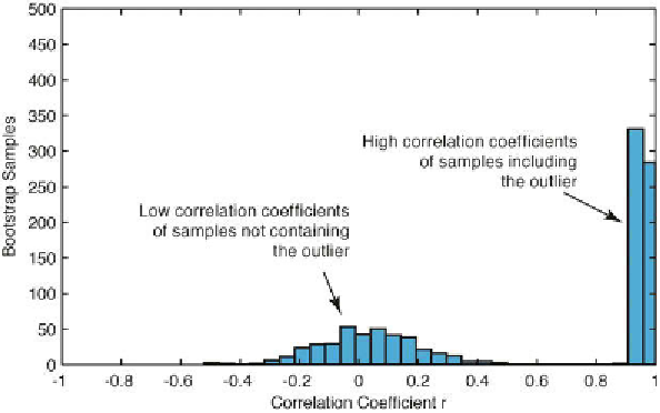
h e histogram shows a cluster of correlation coei cients at around
r
=0.1
that follow the normal distribution, and a strong peak close to
r
=1 (Fig. 4.3).
h e interpretation of this histogram is relatively straightforward. When the
subsample contains the outlier the correlation coei cient is close to one, but
subsamples without the outlier yield a very low (close to zero) correlation
coei cient suggesting the absence of any strong interdependence between
the two variables
x
and
y
.
Bootstrapping therefore provides a simple but powerful tool for either
accepting or rejecting our i rst estimate of the correlation coei cient for the
population. h e application of the above procedure to the synthetic sediment
data yields a clear unimodal Gaussian distribution for the correlation
coei cients of the subsamples.
Fig. 4.3
Bootstrap result for Pearson's correlation coei cient
r
from 1000 subsamples. h e
histogram shows a roughly normally-distributed cluster of correlation coei cients at around
r
=0, suggesting that these subsamples do not include the outlier. h e strong peak close to
r
=1,
however, suggests that an outlier with high values for the two variables
x
and
y
is present in
the corresponding subsamples.