Geoscience Reference
In-Depth Information
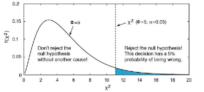
Fig. 3.14
Principles of a ˇ2-test. h e alternative hypothesis that the two distributions are
dif erent can be rejected if the measured ˇ2 is lower than the critical ˇ2. ˇ2 depends on ʦ=
K
-
Z
,
where
K
is the number of classes and
Z
is the number of parameters describing the theoretical
distribution plus the number of variables. In the example the critical ˇ2(ʦ=5, ʱ=0.05) is
11.0705. Since the measured ˇ2= 5.7602 is below the critical ˇ2, we cannot reject the null
hypothesis. In our example we can conclude that the sample distribution is not signii cantly
dif erent from a Gaussian distribution.
clear
corg = load('organicmatter_one.txt');
h = histogram(corg,8);
v = h.BinWidth * 0.5 + h.BinEdges(1:end-1);
n_obs = h.Values;
We then use the function
normpdf
to create the expected frequency distribution
n_exp
with the mean and standard deviation of the data in
corg
.
n_exp = normpdf(v,mean(corg),std(corg));
h e data need to be scaled so that they are similar to the original data set.
n_exp = n_exp / sum(n_exp);
n_exp = sum(n_obs) * n_exp;
h e i rst command normalizes the observed frequencies
n_obs
to a total of
one. h e second command scales the expected frequencies
n_exp
to the sum
of
n_obs
. We can now display both histograms for comparison.
subplot(1,2,1), bar(v,n_obs,'r')
subplot(1,2,2), bar(v,n_exp,'b')
An alternative way of plotting the data in
corg
is to use a normal probability
plot.