Graphics Reference
In-Depth Information
2
B
2
(
t
)=
φ
i
2
(
t
)
v
i
(3.4)
i
=0
=
φ
o
2
(
t
)
v
o
+
φ
12
(
t
)
v
1
+
φ
22
(
t
)
v
2
=(1
−
t
)
2
v
o
+2
t
(1
−
t
)
v
1
+
t
2
v
2
.
3.4.2 Algorithm 1: Approximation Criteria of
f
(
t
)
In order to develop an approximation technique, let us first formulate the key
criteria associated with this technique.
Let us assume
n
-2 quadratic B-B polynomials for the representation of
n
data points such that
f
(
t
i
)=
B
2
i
(
t
i
)
i
=1
,
2
,
3
,
···
,n
−
2
where
B
2
i
(
t
i
) is the value of the
i
th quadratic B-B polynomial at the point
t
i
and is given by
t
i
)
2
v
o
+2
t
i
(1
B
2
i
(
t
i
)=(1
t
i
)
v
1
i
+
t
i
2
v
2
.
−
−
(3.5)
Let
B
2
1
(0) =
B
2
2
(0) =
=
B
2
n−
2
(0) =
v
o
···
and
=
B
2
n−
2
(1) =
v
2
.
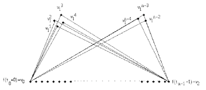
In other words, at the end supports all the quadratic B-B polynomials are
assumed to be identical. The points at end supports are also the vertices of
the underlying
n
-2 polygons. The second vertex (also called the control point)
v
1
i
of the
n
-2 polynomials are all different. This is shown in Figure 3.4.
B
2
1
(1) =
B
2
2
(1) =
···
Fig. 3.4.
Second control points due to a sequence of quadratic polynomials.
From equation (3.5), the second control point of the
i
th polynomial can
be computed as
Search WWH ::

Custom Search