Answers to the Exercises - 3D Math Primer for Graphics and Game Development - page 793

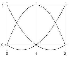
2. We can solve this exercise several ways, but since this is a chapter on curves, we wanted
you to use the polynomial interpolation techniques from Section 13.2 to fit a parabola
through the “control points” given in the problem. Those control points just happen to
share the knot sequence from the previous exercise, and we were hoping you would take
advantage of that work. The math starts by multiplying each Lagrange basis polynomial
by the corresponding control point.

p(t) = p 1 ℓ 1 (t) + p 2 ℓ 2 (t) + p 3 ℓ 3 (t)

(t 2 −3t + 2)/2 +

d/2
h

d
0

0
0

(−t 2 + 2t) + (t 2 −t)/2 =

d/2
h

d
0

(−t 2 + 2t) + (t 2 −t)/2

=

−d/2
−h

d
2h

d/2
0

−d/2
0

t 2 + t 2 +

= t + t

−h d/2

2h

t 2 +

= t

3. (a) Starting with t = 0.4. The first round of interpolation:

b 0 = 0.60 b 0 + 0.40 b 1 = 0.60(3, 5) + 0.40(6, 1) = (4.20, 3.40)
b 1 = 0.60 b 1 + 0.40 b 2 = 0.60(6, 1) + 0.40(0, 3) = (3.60, 1.80)
b 2 = 0.60 b 2 + 0.40 b 3 = 0.60(0, 3) + 0.40(5, 5) = (2.00, 3.80)

Round two:

b 0 = 0.60 b 0 + 0.40 b 1 = 0.60(4.20, 3.40) + 0.40(3.60, 1.80) = (3.96, 2.76)
b 1 = 0.60 b 1 + 0.40 b 2 = 0.60(3.60, 1.80) + 0.40(2.00, 3.80) = (2.96, 2.60)

And the final round:

b 0 = 0.60 b 0 + 0.40 b 1 = 0.60(3.96, 2.76) + 0.40(2.96, 2.60) = (3.56, 2.70)