Game Development Reference
In-Depth Information
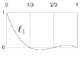
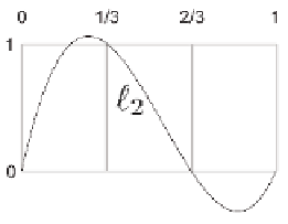
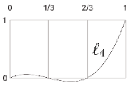
Figure 13.5.
Cubic Lagrange basis polynomials for uniform knot vector
ℓ
2
(t) = (27/2)t
3
− (45/2)t
2
+ 9t,
ℓ
3
(t) = −(27/2)t
3
+ 18t
2
− (9/2)t,
ℓ
4
(t) = (9/2)t
3
− (9/2)t
2
+ t.
Figure 13.5 shows what these basis polynomials look like.
Now that we have the Lagrange basis polynomials for the knot vector,
let's plug in the y values from our example S curve (
Figure 13.2)
into
Equation (13.7) to get the complete interpolating polynomial:
P(t) = y
1
ℓ
1
(t) + y
2
ℓ
2
(t) + y
3
ℓ
3
(t) + y
4
ℓ
4
(t)
= 2[−(9/2)t
3
+ 9t
2
− (11/2)t + 1] + 3[(27/2)t
3
− (45/2)t
2
+ 9t]
+ 2[−(27/2)t
3
+ 18t
2
− (9/2)t] + 3[(9/2)t
3
− (9/2)t
2
+ t]
= −9t
3
+ 18t
2
− 11t + 2 + (81/2)t
3
− (135/2)t
2
+ 27t
− 27t
3
+ 36t
2
− 9t + (27/2)t
3
− (27/2)t
2
+ 3t
= 18t
3
− 27t
2
+ 10t + 2.
Let's show these results graphically. First, we scale each basis polyno-
mial by the corresponding coordinate value, as shown in
Figure 13.6.
Finally, adding the scaled basis vectors together yields the interpolating
polynomial P, the blue curve at the top of
Figure 13.7.


Search WWH ::

Custom Search