Curves in 3D - 3D Math Primer for Graphics and Game Development - page 655

t x(t) y(t)

0 0 2

1/3 1/3 3

2/3 2/3 2

1 1 3

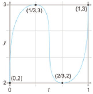
Figure 13.2. An example curve and four control points. Can we draw this shape?

that the knot vector is the sequence of t values, not the sequence of control
points.)
What about the x-coordinate? Because the x and y coordinates are
independent of one another, a general 2D curve-fitting application involves
two separate one-dimensional problems. Aside from the fact that the two
problems use the same knot vector, the coordinates are otherwise unrelated.
Even though Figure 13.2 may look like a 2D curve, it is more properly
interpreted as a graph of one coordinate (the y-coordinate) as a function of
time. We chose as the example curve an S turned on its side, rather than
an S in its regular orientation, since the latter is not the graph of a function
(technically it's called a relation because it associates more than one value
of y with each value of x).
With that said, there are two ways of interpreting Figure 13.2. We can
interpret it either as a 1D function of y(t), or as a 2D curve, where one of the
coordinates has a trivial form x = t. This is a common source of confusion
when looking at diagrams of curves in this topic and elsewhere. Make sure
you pay special attention to the horizontal axis to make sure you know
whether it is a graph of one coordinate over time or a plot of the 2D curve
that includes the behavior of both spatial coordinates. The traditional
literature on polynomial interpolation is mostly in abstract terms of any
function of the form y = f(x). In this context, x would be the independent
variable rather than a dependent value as it is for us. The notation we have
chosen avoids the symbol x and its associated baggage.
Now we are ready to answer a question some readers might be think-
ing: “I don't care what time the curve reaches the points, I just want a