Global Positioning System Reference
In-Depth Information
with covariance matrix
R
(
t
n
). The Kalman filter, once processing is initiated, alter-
nates between two sets of equations describing: (1) the extrapolation of estimate
and error covariance between measurements, and (2) the incorporation of the new
measurements into the estimate. The state estimate extrapolation is given by
()
()
(
)
$
−
$
+
x
t
=
t
,
t
x
t
n
n
n
−
1
n
−
1
and the error covariance extrapolation is given by
()
()
(
(
)
)
(
)
P
t
−
=
t
,
t
P
t
+
T
t
,
t
+
Q
t
n
n
n
−
1
n
−
1
n
n
−
1
n
−
1
The state estimate measurement update is given by
[
]
() ()
()
()
()()
$
$
$
+
−
−
x
t
=
x
t
+
K
t
y
t
−
H
t
x
t
n
n
n
n
n
n
where
K
(
t
n
) is the Kalman gain matrix and is computed by
[
]
()
() ()
()
−
1
()
() ()
−
T
−
T
K
t
=
P HHP H R
t
t
t
t
t
+
t
n
n
n
n
n
n
n
The error covariance update is
()
[
] ()
()()
+
−
P
t
=−
I K
t
H
t
P
t
n
n
n
n
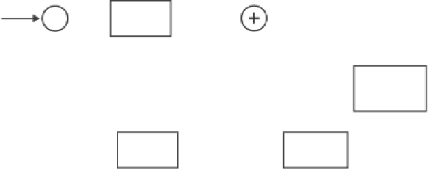
Figure 9.7 shows the Kalman filter processing scheme.
In practice, one is concerned with the computational issues arising from the use
of finite precision in computers. If care is not taken, the filter can become unstable,
and the solution diverges from the correct values. In inertial navigation systems,
where a full model may require up to 60 states, much analysis is placed on proper
selection of the critical states to produce what is called a suboptimal Kalman filter,
which is computationally well behaved. Also of concern are wraparound errors
(i.e., in 16-bit systems 32,767
32,768), which may cause a complete reversal
on signs and round off errors [7, 8]. One modification seen in filters used with iner-
tial systems is the use of the filter to determine the error in the state. By setting the
initial estimate of the state to zero and inputting the observed error in the state for
+
1
=−
y
()
t
n
x
()
t
n
+
+
K
()
t
n
Optimal
estimate
−
x
()
t
n
−
Delay
x
()
t
n
−
H
()
t
n
(,
t
n
t
n
−
1
)
x
(
t
n
−
1
)
Figure 9.7
Kalman filter processing scheme.


Search WWH ::

Custom Search