Global Positioning System Reference
In-Depth Information
2
()
t
−
σ
xn
Delay
σ
x
2
(
2
()
t
+
)=[1
k t
( )]
t
−
−
σ
xn
n
n
2
()
σ
xn
t
−
k
()=
n
Kalman gain
computation
2
2
( +
t
−
σ
σ
xn
m
k
(
n
Optimal
estimate
xt
()=
n
+
xt
( )+( [()
−
kt
yt
xt
( ]
−
−
y
(
n
+
kyt
[( )
xt
(
−
)]
−
n
n
n
n
n
n
X
−
xt
()
n
−
Estimator
Delay
xt
()
n
−
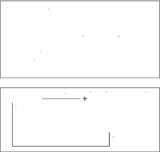
Figure 9.6
Basic Kalman filter.
be extrapolated to the next measurement time according to the system state model
to compute
xt
n
−
1
. Also, in the more general vector case, the performance of the
Kalman filter estimate is characterized by an error covariance matrix denoted as
P
(
t
n
) and defined by
$
(
)
()
(
() ()
)
(
() ()
)
T
$
$
P
t
=
E
x
t
−
x
t
x
t
−
x
t
n
n
n
n
n
Here we summarize the Kalman filter equations for the general case. The state
system model is given by
()
(
)( ) ()
x
t
=
t
,
t
x
t
+
u
t
n
n
n
−
1
n
−
1
n
where
(
t
n
,
t
n
−1
) denotes the system one-step transition matrix, and
u
(
t
n
) is the plant
or process noise vector that is assumed to be white, zero mean, and distributed nor-
mally. This is represented by the function N(0,
Q
(
t
n
)) with covariance matrix
Q
(
t
n
).
The measurement model is
Φ
()
()()
()
y Hx
t
=
t
t
+
t
n
n
n
m
n
where
y
(
t
n
) is a vector, and the measurement matrix
H
(
t
n
) characterizes the sensitiv-
ity of the measurements to each of the state components. Vector
m
(
t
n
) is the mea-
surement noise and is a white random process distributed normally as N(0,
R
(
t
n
))


Search WWH ::

Custom Search