Integration of GPS with Other Sensors and Network Assistance - Understanding GPS: Principles and Applications - page 462

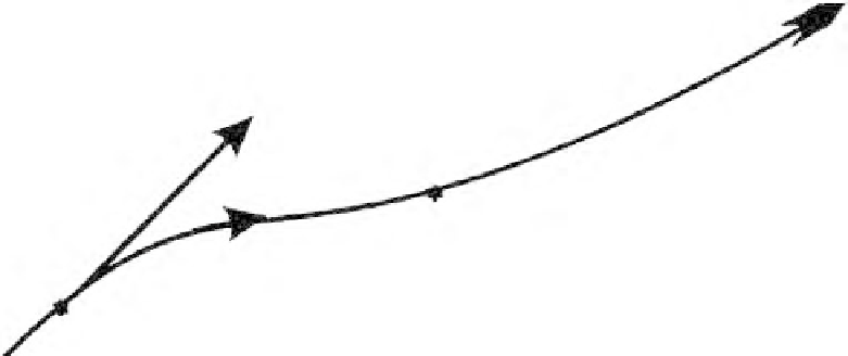
Vehicle path

Estimated position and
velocity between updates

GPS position/velocity
update

Actual position and velocity between updates

GPS position/velocity update

Figure 9.2 Extrapolation of GPS navigation solution in a dynamic environment.

tion filter can be used to reduce the time to reacquire GPS signals that have been lost
through interference or obscuration; second, the integration filter can be used to aid
the receiver's tracking loops, extending the thresholds for signal tracking. Both tech-
niques have been used since the very first GPS sets were designed [1]. The first
enhancement, often referred to as prepositioning , computes an a priori estimate of a
signal's code phase and Doppler using the integration filter's estimates of position
and velocity, and time and frequency error. If the combined position and timing
errors are less than one-half a chip (roughly 150m for the C/A code, and 15m for the
P(Y) code), then nearly instantaneous reacquisition of a lost signal is possible, since
the prepositioning limits the tracking error to the linear range of the loop's error
detector (see Section 5.4 ) . Similarly, Doppler on the signal to be reacquired can be
predicted from the integration filter's estimates of velocity and signal frequency, and
if those estimates are within the linear range of the frequency error detector (see Sec-
tion 5.3.3), nearly instantaneous signal acquisition may be possible. For example, if
using an arctangent error detector with a 5-ms predetection integration interval
(PDI), the combined frequency error can be as large as 50 Hz, which translates to a
velocity accuracy of 10 m/s, which is readily achievable using a navigation grade
IMU and potentially achievable with tactical grades [2]. Generally speaking, if the
navigation filter is a “robust design” (i.e., its covariance matrix is consistent with the
error in its navigation solution), then the uncertainty associated with the predicted
code phase and Doppler is best determined from the covariance matrix. For exam-
ple, if P 4 represents the 4 × 4 partition of the filter's covariance matrix corresponding
to position and time error, then the error variance associated with a predicted code
phase can be computed using:

2

σ cp = hPh

T

(9.1)

4

In (9.1), h is the filter's measurement gradient vector to the satellite of interest,
comprised of the LOS unit vector to the satellite of interest (first three elements) and
the sensitivity of the user's clock phase error (fourth element). Generally, the ele-
ments of the covariance matrix P 4 in (9.1) are expressed in units of m 2 . In this case,
the code phase error variance σ cp 2 will also be expressed in m 2 . Given the error vari-