Model-Based Segmentation, Reconstruction and Analysis of the Vertebral Body from Spinal CT - Spinal Imaging and Image Analysis - page 412

Table 5 Graph edges
weights

Edge Weight For

f p ; q g V ð f p ; f q Þ f p ; q g2N

cm f s ; p g log½P ð I p j 1 Þ P ð d p j 1 Þ p 2V

1 p 2O

0 p 2B

cm f p ; t g log½P ð I p j 0 Þ P ð d p j 0 Þ p 2V

0 p 2O

1 p 2B

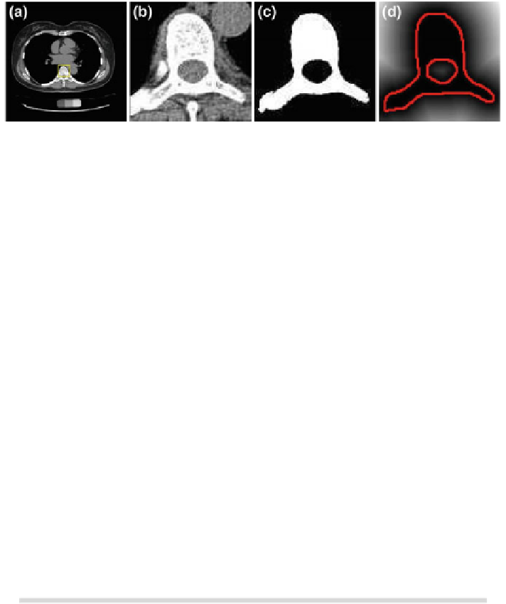
Fig. 34 An example of the initial labeling. a A CT slice of vertebral body. (yellow box illustrates
detected VB region). b Detection of the VB region. c The initial labeling, f . d The SDF of the
initial segmentation which is used in the registration phase (see Algorithm 3). Red color shows the
zero level contour

Algorithm 3 Given: The input VB set of images, the ESP (J as a source
information), the probabilistic 3D shape model (d).
Objective: To obtain the desired labeling (f) using the required transfor-
mation matrix (T).

1. Detect the VB region using [ 40 ]
2. Obtain the initial segmentation (f ) using graph cuts which integrates the
intensity and spatial interaction models only.
3. Register the shape prior to the initially segmented volume. J and f will be
the source and target information, respectively. After the transformation,
the embedded shape model and its features are described as follows:

After each voxel p 2P s is transformed to the new voxel b p, the shape

￿

new , new , and

model is registered to the volume domain. We obtain new O B

new

V :

The object/variability surface C new
OV

is updated as well.

￿

Hence, new iso-surfaces at the same distances, they have the same
probabilistic distance value with the iso-surfaces which are obtained

￿