Information Technology Reference
In-Depth Information
9
includes the center, orientation and size of the disc. It is worth noting that i is
not a simple index but bears anatomical de
d
i
2
R
nition. In this paper, without loss of
generality, v
i
is indexed in the order of vertebrae from head to feet, e.g., v
1
, v
24
, v
25
represents C
1
, L
5
and S
1
, respectively.
Formulation: Given an image I, spine detection problem can be formulated as
the maximization of a posterior probability with respect to V and D as:
V
;
D
Þ
¼
ð
argmax
V
;
D
P
ð
V
;
D
j
I
Þ
ð
1
Þ
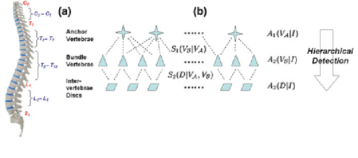
Certain vertebrae that appear either at the extremity of the entire vertebrae column,
e.g., C
2
, S
1
, or at the transition regions of different vertebral sections, e.g., L
1
, have
much better distinguishable characteristics (red ones in Fig.
2
a). The identi
cation
of these vertebrae helps in the labeling of others, and are de
ned as
“
anchor
vertebrae
. The remaining vertebrae (blue ones in Fig.
2
a) are grouped into a set of
continuous
”
. Vertebrae char-
acteristics are different across bundles but similar within a bundle, e.g., C
3
-
“
bundles
”
and hence de
ned as
“
bundle vertebrae
”
C
7
look
similar but are very distinguishable from T8-T12.
8
-
T
12
.
Denoting V
A
and V
B
as anchor and bundle vertebrae, the posterior in Eq. (
1
) can
be rewritten and further expanded as:
P
ð
V
;
D
j
I
Þ
¼
P
ð
V
A
;
V
B
;
D
j
I
Þ
¼
P
ð
V
A
j
I
Þ
P
ð
V
B
j
V
A
;
I
Þ
P
ð
D
j
V
A
;
V
B
;
I
Þð
2
Þ
In this study, we use Gibbs distributions to model the probabilities. The logarithm
Eq. (
2
) can be then derived as Eq. (
3
).
log
½
P
ð
V
;
D
j
I
Þ
¼
A
1
ð
V
A
j
I
Þ
(
P
ð
V
A
j
I
Þ
þ
A
2
ð
V
B
j
I
Þþ
S
1
ð
V
B
j
V
A
Þ (
P
ð
V
B
j
V
A
;
I
Þ
ð
3
Þ
þ
A
3
ð
D
j
I
Þþ
S
2
ð
D
j
V
A
;
V
B
Þ(
P
ð
D
j
V
A
;
V
B
;
I
Þ
Fig. 2 a Schematic explanation of anchor (red) and bundle (blue) vertebrae. b Proposed spine
detection framework