Information Technology Reference
In-Depth Information
here w and b are separating plane parameters, and
/ð
x
Þ
is a function to map vector
T
x into a higher dimensional space. K
is called the kernel
function. We are using radial basis functions as the kernel function, i.e.
ð
x
i
;
x
j
Þ
¼
/ð
x
i
Þ
/ð
x
j
Þ
2
K
ð
x
i
;
x
j
Þ
¼exp
x
i
x
j
ð
24
Þ
To separate two training classes, SVM is employed to solve the following
optimization problem:
!
C
X
N
1
2
w
T
w
min
w
;
b
;f
þ
n
i
ð
25
Þ
i¼1
w
T
/ð
subject to
y
i
ð
x
i
Þþ
b
Þ
1
n
i
;
n
i
0
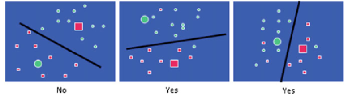
here C is the penalty parameter. The mechanism of SVM is illustrated in Fig.
7
,
where a hyperplane is
fit to separate two groups of dots. SVM allows a soft margin
on each side of the hyperplane. For each data point, the distance to the margin of
hyperplane is computed. If the point is on the correct side of the plane, the distance
is 0. The optimization process is to minimize the total distance of all training points.
After the hyperplane is determined, the decision function for the classi
cation rule
can be written as
h
ð
x
Þ
¼
signðf
ð
f
ð
x
ÞÞ
ð
26
Þ
ed based on which side of the hyperplane it lies, i.e.,
it is declared a metastasis if h(x) > 0, or a non-metastasis if h(x) < 0. The feature
values in SVM are normalized to the range of [
A new detection x, is classi
1, +1]. The normalization factor is
obtained from the training data and applied to the testing data.
An SVM in higher dimensional space (more features) can lead to more accurate
classi
−
cation. However, SVM in a very high dimensional space may increase the
complexity of the model, over-train the data and decrease the generality of the
model. One solution is to use an ensemble of classi
ers, in which each classi
er
includes a small number of features.