Graphics Reference
In-Depth Information
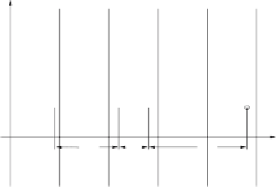
Figure
.
.
(Let) he two points at which the lines intersect uniquely determine a plane π in
-D.
(Right) he coe
cients of π
c
can be read from the picture produced by four
points that are similarly constructed by consecutive axis translations!
c
x
+
c
x
+
c
x
=
for S
c
.he three subscripts correspond to the three variables that appear
in the equation of the plane, and distinguish them from the points with two sub-
scripts, which represent lines. he second and third axes can also be consecutively
translated, as indicated in Fig.
.
(let), repeating the construction togenerate two
more points denoted by π
′
′
, π
′
′
′
. hese points can also be found in another, eas-
ier,way.hegistofallthisisshowninFig.
.
(right).hedistancebetween succes-
sive points is
c
i
.heequationoftheplaneπ can actually be read from the picture!
In general, a hyperlane in N dimensions is represented uniquely by N
=
c
+
c
+
points,
each with N indices. here is an algorithm that constructs these points recursively,
raising the dimensionality by one at each step, as is done here starting from points
(zero-dimensional) and constructing lines (one-dimensional). By the way, all of the
nicehigh-dimensionalprojectivedualities,like point
−
hyperplane,rotation
trans-
lation,etc., hold.Further,a multidimensional object represented in
-coordscan still
be recognized ater it has been acted on by projective transformation (i.e., transla-
tion, rotation, scaling andperspective). herecursive construction andits properties
are at the heart of the
-coords visualization.
Challenge: Visualizing Families of Proximate Planes
Returningto
-D,itturnsoutthatforpointslikethoseinFig.
.
whichare“nearly”
coplanar (i.e., have small errors), the construction produces a pattern that is very
similar to that in Fig.
.
(let). A little experiment is in order. Let us return to the
family of proximate (i.e., close) planes generated by
c
−
i
, c
+
Π
=
π
c
x
+
c
x
+
c
x
=
c
, c
i
[
]
, i
=
,
,
,
(
.
)
i
We randomly choose values for c
i
within the allowed intervals to determine a plane
π
initially, and then we plot the two points π
, π
′
as shown
in Fig.
.
(let). Closeness is apparent, and more significantly the distribution of
Π, keeping c
=