Graphics Reference
In-Depth Information
Figure
.
.
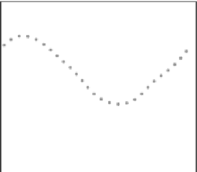
he let-hand panel shows a smooth curve as an estimate of the underlying regression
function for the seasonal effect in the Clyde data, with variability bands to indicate the precision of
estimation. he dotted line denotes a smoothed version of a shited and scaled cosine model. he
right-hand panel shows an estimate of the year effect ater adjustment for the seasonal effect.
A reference band has been added to indicate where a smooth curve is likely to lie if the underlying
relationship is linear
A natural model for the seasonal effect is a shited and scaled cosine curve, of the
form
(
x
i
−
θ
)
y
i
=
α
+
β cos
π
+
ε
i
,
where the smaller effect across years, if present at all, is ignored at the moment. Mc-
Mullan et al. (
) describe this approach. A simple expansion of the cosine term
allows this model to be written in simple linear form, which can then be fitted to be
observed data very easily.
However, some thought is required in comparing a parametric form with a non-
parametric estimate. As noted above, bias is an inevitable consequence of nonpara-
metric smoothing. We should therefore compare our nonparametric estimate with
whatweexpecttoseewhenanonparametricestimateisconstructedfromdatagener-
atedbythecosinemodel.hiscaneasilybedonebyconsidering E
,wherethe
expectation is calculated under the cosine model. he simple fact that
E
m
(
x
)
suggests that we should compare the nonparametric estimate Sy
with a smoothed version of the vector of fitted values y from the cosine model,
namely S y.hiscurvehasbeenaddedtothelethandplotofFig.
.
anditagreesvery
closely with the nonparametric estimate. he cosine model can therefore be adopted
as a good description of the seasonal effect.
Since the seasonal effect in the Clyde data is so strong, it is advisable to reexam-
ine the year effect ater adjustment for this. Nonparametric models involving more
than one covariate will be discussed later in the chapter. For the moment, a simple
expedient is to plot the residuals from the cosine modelagainst year, as shown in the
right hand panel of Fig.
.
. he reduction in variation over the marginal plot of DO
against year is immediately apparent.
Sy
=
SE
y