Graphics Reference
In-Depth Information
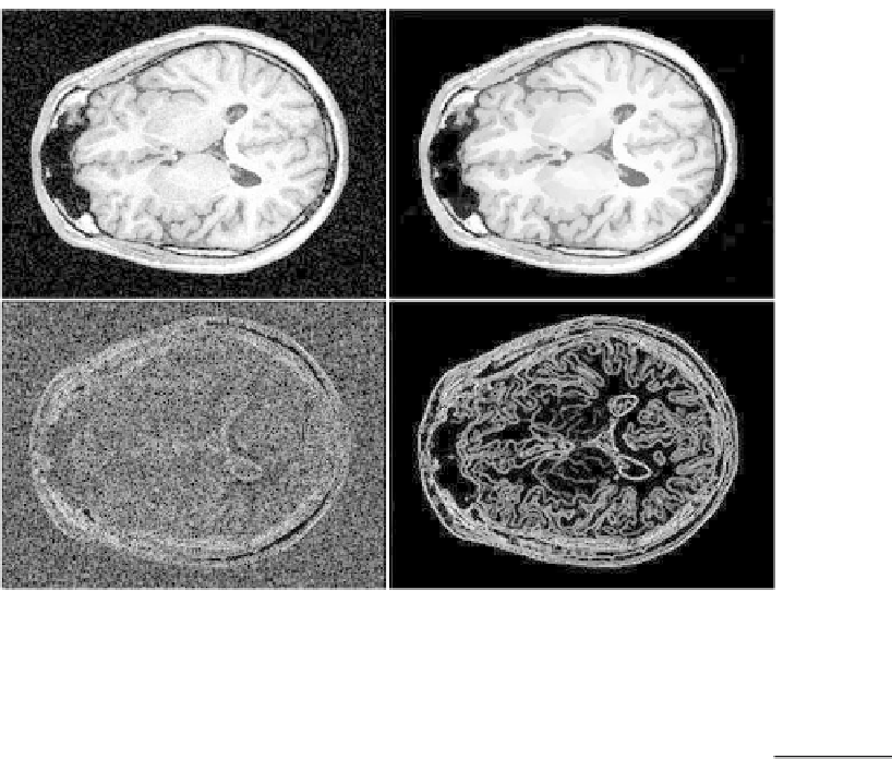
Figure
.
.
-D Magnetic resonance imaging (MRI): Slice
from a
-D MR image (upper let)andits
-D reconstruction by AWS (upper right). he bottom row shows the result of applying an edge
detection filter to both images
Examples: Binary and Poisson Data
8.4.2
For non-Gaussian data, the stochastic penalty s
ij
takes a different form in (
.
).
he definition is based on the Kullback-Leibler distance
K
between the probability
measures P
θ
i
and P
θ
j
. For binary data this leads to
(
k
−)
i
θ
(
k
−)
i
θ
(
k
−)
i
N
log
−
θ
θ
(
k
)
ij
(
k
−)
i
(
k
−)
i
s
=
log
+(
−
)
(
.
)
λ
θ
(
k
−)
j
θ
(
k
−)
j
−
while for Poisson data we get
θ
(
k
−)
i
(
k
−)
i
N
θ
θ
θ
(
k
)
ij
(
k
−)
i
(
k
−)
i
(
k
−)
j
s
=
log
−
+
.
(
.
)
θ
λ
(
k
−)
j
In both cases a special problem occurs. If the estimates θ
i
or θ
j
attain a value at the
boundary oftheparameter space,i.e.,
or
forbinary data or
inthecase ofPoisson
data, then the Kullback-Leibler distance between the probability measures P
θ
i
and
P
θ
j
will equal
. Such a situation can be avoided by modifying the algorithm. One
solution is to initialize the estimates with the value obtained by the global estimate