Graphics Reference
In-Depth Information
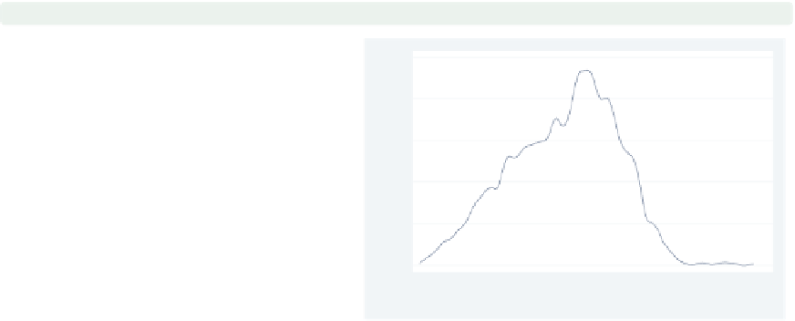
twoway kdensity ttl exp,
biweight
By default, Stata uses a Epanechnikov
kernel for computing the density
estimates. Here, we use the
biweight
option to use the biweight kernel for
computing the densities. Other
methods include
cosine
,
gauss
,
parzen
,
rectangle
,and
triangle
.
Uses nlsw.dta & scheme vg s2c
0
10
20
30
x
twoway kdensity ttl exp,
range(0 40)
You can use the
range()
option to
specify the range of the
-values at
which the kernel density is computed
and displayed. Here, we expand the
rangetospanfrom0to40.
Uses nlsw.dta & scheme vg s2c
x
0
10
20
30
40
x
twoway (histogram ttl exp, width(1) frequency)
(kdensity ttl exp,
area(2246)
)
In this example, we overlay a histogram
of
ttl exp
, scaling the
-axis as the
frequency of values in each bin. We
overlay this with a
kdensity
plot but
want to scale the
y
-axis in a
commensurate manner. By using the
area()
option, we can specify that the
sum of the area of the kernel density
should sum to 2246, the sample size.
Uses nlsw.dta & scheme vg s2c
y
0
10
20
30
Frequency
kdensity ttl_exp, area=2246
The electronic form of this topic is solely for direct use at UCLA and only by faculty, students, and staff of UCLA.