Graphics Reference
In-Depth Information
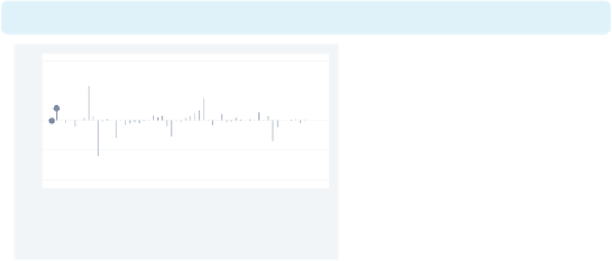
twoway (rspike hi low date) (rcap close close date, msize(medsmall))
(scatteri 1220 15027 1220 15034, recast(line) clwid(vthick) clcol(red)),
tlabel(08jan2001 01feb2001 21feb2001) legend(off)
This example is the same as above,
except that this one uses
scatteri()
to
draw a support-level line. Two
pairs
are given after the
scatteri
, and the
recast(line)
option draws them as a
line instead of two points. The
yx
-values
were calculated beforehand using
display d(21feb2001)
and
display d(28feb2001)
to compute the
elapsed date values.
Uses spjanfeb2001.dta & scheme
vg samec
x
08jan2001
01feb2001
21feb2001
The rest of the examples in this section involve some data management before we create
the graph. For the next few examples, we use the
allstates
data file and run a regression
command,
. vguse allstates
. regress ownhome propval100 workers2 popden
and then issue the
. dfbeta
command, creating
DFBETA
s for each predictor:
DFpropval100
,
DFworkers2
,and
DFurban
,
which are used in the following graph.
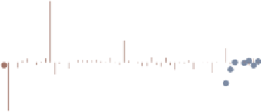
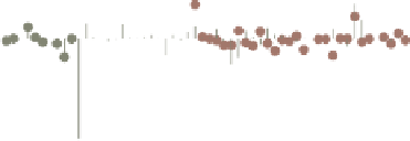
twoway dropline DFpropval100 DFworkers2 DFurban statefips,
mlabel(stateab stateab stateab)
In this example, we show each of the
DFBETA
sasa
dropline
plot. We add
the
mlabel()
option to label each point
with the state abbreviation.
Uses allstates.dta & scheme vg s2c
DC
CT
MN
MM
M
NN
N
N
N
N
N
N
OO
O
PA
R
SC
SD
NJ
N
N
N
N
O
O
O
PARS
S
T
TX
UT
UT
VT
VA
W
W
W
WY
UT
V
VAW
W
W
WY
AK
A
A
C
CO
F
G
HI
I
I
I I
KK
L
ME
M
M
M
N
N
NH
A
A
A
A
C C
CT
M
M
M
M
MM
M
NE
N
NH
N
N
O
O
O
PARS
S
T
TX
I
I I I KK
LM
M
M
MI
I
I
I
I K
K
L
M
M
M
A
N
N
NY
A
A
C
C
C
DE
D
E
F
GA
HI
V
VA
W
W
W
W
Y
DE
TTX
AL
G
H
I
AL
MI
MN
FL
DC
AK
DC
0
20
40
60
state code
Dfbeta propval100
Dfbeta workers2
Dfbeta urban
The electronic form of this topic is solely for direct use at UCLA and only by faculty, students, and staff of UCLA.