Graphics Reference
In-Depth Information
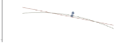
twoway (scatter ownhome urban) (lfit ownhome urban) (qfit ownhome urban),
legend(order(- "Fitted" 2 "Lin.
fit" 3 "Quad.
fit" - "Observed" 1)
cols(1)
)
We can use the
cols()
option to
display the legend in a single column.
Here, the added text makes more sense,
but the legend uses quite a bit of space.
Uses allstatesdc.dta & scheme vg s2c
20
40
60
80
100
Percent urban 1990
Fitted
Lin. fit
Quad. fit
Observed
% who own home
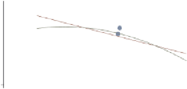
twoway (scatter ownhome urban) (lfit ownhome urban) (qfit ownhome urban),
legend(order(- "Fitted" 2 "Lin.
fit" 3 "Quad.
fit" - "Observed" 1)
rows(3)
)
We can use the
rows()
option to
display the legend in three rows. If we
want to display the fitted keys in the
left column and the observed keys in
the right column, we can order the keys
according to columns instead of
according to rows. See the next
example.
Uses allstatesdc.dta & scheme vg s2c
20
40
60
80
100
Percent urban 1990
Fitted
Lin. fit
Quad. fit
Observed
% who own home
twoway (scatter ownhome urban) (lfit ownhome urban) (qfit ownhome urban),
legend(order(- "Fitted" 2 "Lin.
fit" 3 "Quad.
fit" - "Observed" 1)
rows(3)
colfirst
)
Adding the
colfirst
option displays
the keys in column order instead of row
order, with the Fitted keys in the left
column and the Observed keys in the
right column.
Uses allstatesdc.dta & scheme vg s2c
20
40
60
80
100
Percent urban 1990
Fitted
Lin. fit
Quad. fit
Observed
% who own home
The electronic form of this topic is solely for direct use at UCLA and only by faculty, students, and staff of UCLA.