Graphics Reference
In-Depth Information
twoway (scatter ownhome urban if north==0)
(scatter ownhome urban if north==1)
A third example is when you overlay
two plots using
if
to display the same
variables but for different observations.
Here, we show the same scatterplot
separately for states in the North and
for those not in the North. Here, the
legend does not help us at all to
differentiate the kinds of values.
Uses allstatesdc.dta & scheme vg s2c
20
40
60
80
100
Percent urban 1990
% who own home
% who own home
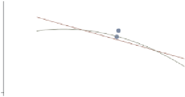
twoway (scatter ownhome urban) (lfit ownhome urban)
(qfit ownhome urban)
Regardless of the graph command(s)
that generated the legend, it can be
customized the same way. For many of
the examples, we will use this graph for
customizing the legend.
Uses allstatesdc.dta & scheme vg s2c
20
40
60
80
100
Percent urban 1990
% who own home
Fitted values
Fitted values
twoway (scatter ownhome urban) (lfit ownhome urban)
(qfit ownhome urban),
legend(
label(1 "% Own home") label(2 "Lin.
Fit") label(3 "Quad.
Fit")
)
You can use the
label()
option to
assign labels for the keys. Note that
you use a separate
label()
option for
each key that you wish to modify.
Uses allstatesdc.dta & scheme vg s2c
20
40
60
80
100
Percent urban 1990
% Own home
Lin. Fit
Quad. Fit
The electronic form of this topic is solely for direct use at UCLA and only by faculty, students, and staff of UCLA.