Graphics Reference
In-Depth Information
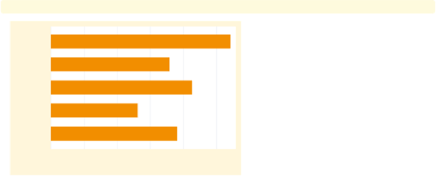
graph hbar wage,
over(occ5)
Here, we use the
over()
option to show
the average wages broken down by
occupation. Note that we are using
graph hbar
to produce horizontal,
rather than vertical, bar charts.
Uses nlsw.dta & scheme vg brite
Prof/Mgmt
Sales
Clerical
Labor/Ops
Other
0
2
4
6
8
10
mean of wage
graph hbar wage, over(occ5)
over(collgrad)
Here, we use the
over()
option twice to
show the wages broken down by
occupation and whether one graduated
college. Note the appropriate way to
produce this graph is to use two
over()
options, rather than using a single
over()
option with two variables. As
we will see later, each
over()
can have
its own options, allowing you to
customize the display of each
over()
variable.
Uses nlsw.dta & scheme vg brite
Prof/Mgmt
Sales
not college grad
Clerical
Labor/Ops
Other
Prof/Mgmt
Sales
college grad
Clerical
Labor/Ops
Other
0
5
10
15
mean of wage
graph hbar wage,
over(urban2)
over(occ5) over(collgrad)
We can even add a third
over()
option, in this case using
over(urban2)
to compare those living in rural versus
urban areas. Note the change in the
look of the graph when we add the
third
over()
variable. This is because
Stata is now treating the first
over()
variable as though it were multiple
y
Prof/Mgmt
Sales
not college grad
Clerical
Labor/Ops
Other
Prof/Mgmt
Sales
college grad
Clerical
Labor/Ops
Other
-variables. Because of this, you can
only specify one
-variable when you
have three
over()
options.
Uses nlsw.dta & scheme vg brite
y
0
5
10
15
mean of wage
Rural
Metro
The electronic form of this topic is solely for direct use at UCLA and only by faculty, students, and staff of UCLA.