Graphics Reference
In-Depth Information
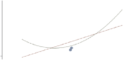
twoway (scatter propval100 urban) (lfit propval100 urban)
(qfit propval100 urban,
legend(label(2 Linear Fit) label(3 Quad Fit))
)
We can make the previous graph in a
different, but less appropriate, way.
The
legend()
option is given as an
option of the
qfit()
command, not at
the very end as in the previous graph
command. But Stata is forgiving of
this, and even when such options are
inappropriately given within a
particular command, it treats them as
though they were given at the end of
the command.
Uses allstates.dta & scheme vg teal
100
80
60
40
20
0
20
40
60
80
100
Percent urban 1990
% homes cost $100K+
Linear Fit
Quad Fit
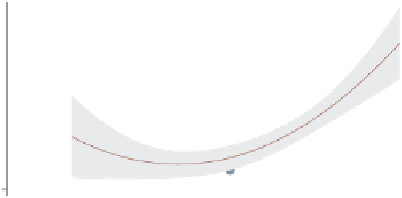
twoway (
qfitci
propval100 urban) (
scatter
propval100 urban)
Another common example of overlaying
graphs is to overlay a fit line with
confidence interval and a scatterplot.
Uses allstates.dta & scheme vg teal
100
80
60
40
20
0
20
40
60
80
100
Percent urban 1990
95% CI
Fitted values
% homes cost $100K+
twoway (
scatter
propval100 urban) (
qfitci
propval100 urban)
However, note the order in which you
overlay these two kinds of graphs. In
this example, the
qfitci
was drawn
after the
scatter
, and as a result, the
points are obscured by the confidence
interval.
Uses allstates.dta & scheme vg teal
100
80
60
40
20
0
20
40
60
80
100
Percent urban 1990
% homes cost $100K+
95% CI
Fitted values
The electronic form of this topic is solely for direct use at UCLA and only by faculty, students, and staff of UCLA.