Biomedical Engineering Reference
In-Depth Information
1.2
1
0.8
0.6
0.4
0.2
0
1 2 3 4 5 6 7 8 91011121314151617
Iteration Number
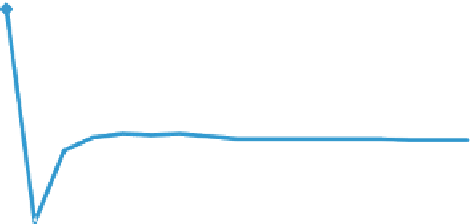
FIGURE 4.6
Iteration history for the cost function.
measure. This cost function will be optimized to predict the motion. Note that
this example serves as an introduction to the following chapter, “Predictive
dynamics,” which is the essence of this topic.
Consider an energy consumption cost function defined as
ð
T
!
dt
u
X
n
i
5
1
τ
2
i
ð
1
uÞ
1
u
A½
0
;
1
(4.99)
2
t
5
0
where
u
is a specified constant and
T
is the total travel time of the arm. The second
term, torque square, is related to energy consumption. When
u
goes to zero, this cost
function becomes the time-optimal criterion. An appropriate
u
avoids harsh func-
tioning of the actuator torques (
Bessonnet and Lallemand, 1990
). We shall also add
an external load to the arm as if it is carrying a load from one point to another.
We shall use the same example treated earlier of the two-link arm with physi-
cal parameters as listed in
Table 4.1
. The constant vertical external load
f
5
10 N
acting at the hand and the gravity effect
g
9
:
8062
m
=
s
2
are considered in this
5
case. The optimization formulation is given as follows:
!
dt
u
X
n
i
5
1
τ
Ð
t
5
0
2
Min
:
ð
1
uÞ
1
i
ð
x
Þ
u
A½
0
;
1
2
St
:
q
1
ð
0
Þ
5
1
:
32
;
q
2
ð
0
Þ
52
2
:
37
(4.100)
q
1
ðTÞ
5
2
:
80
;
q
2
ðTÞ
52
2
:
37
q
1
ð
0
Þ
5
_
_
q
2
ð
0
Þ
5
_
q
1
ðTÞ
5
_
q
2
ðTÞ
5
0
:
0
#
τð
x
Þ
#
2
10
10
where
is a vector of control points P (joint profile) and total time
T
:
x
5
½P
;
T
.
x
u
01. Starting points are obtained by linear interpolation between the initial
and final joint angles.
0
:
5


Search WWH ::

Custom Search